First Degree Stochastic Dominance
Risky asset A is said to dominate risky asset B in the sense of First Degree Stochastic Dominance (FSD), denoted as \( A \succeq_{FSD} B \), if every individual with a utility function that is increasing and continuous in wealth either prefers A over B or is indifferent between them.
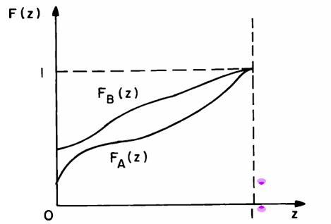
The underlying intuition is straightforward: if, for every level of return \( z \in [0,1] \), the probability that A gives a return less than \( z \) is less than or equal to that of B, then A is considered better. In other words:
\[ F_A(z) \leq F_B(z) \quad \text{for all } z \in [0,1], \] where \( F_A(\cdot) \) and \( F_B(\cdot) \) are the cumulative distribution functions (CDFs) of returns on assets A and B, respectively.
Since the CDF gives the probability that a return is less than or equal to a certain value, the inequality \( F_A(z) \leq F_B(z) \) means that A tends to deliver higher returns more often than B. Thus, any nonsatiable (strictly increasing utility) individual would prefer A.
Properties and Assumptions
We assume:
- The returns of A and B lie in the interval \([0,1]\).
- The CDFs \( F_A(\cdot) \) and \( F_B(\cdot) \) are right-continuous and satisfy \( F_A(1) = F_B(1) = 1 \).
- They may have different masses at zero: \( F_A(0) \neq F_B(0) \).
Interpretation
Condition \( F_A(z) \leq F_B(z) \) for all \( z \) implies that:
- The probability that A returns less than \( z \) is lower than B’s.
- Equivalently, the probability that A returns more than \( z \) is higher than B’s.
Illustrative Example
Suppose assets A and B can each take on the values 0, \( \frac{1}{2} \), and 1. Let the cumulative probabilities (from Figure 1) be such that for each level \( z \in \{0, \frac{1}{2}, 1\} \), the condition \( F_A(z) \leq F_B(z) \) is satisfied.
For example, even though A satisfies FSD over B, it is possible that in one realization A yields 0 while B yields 1. If A and B are independent, the probability of this particular event might be 0.05. So ex post, B may outperform A, but ex ante, A is preferred under FSD.
The concept of FSD thus captures a strong form of dominance: A is better for every decision maker whose preferences are increasing in wealth. This condition is both necessary and sufficient for FSD.
Characterization of First-Order Stochastic Dominance (FSD)
A more intuitive characterization of First-Order Stochastic Dominance (FSD) is based on the idea of comparing one asset’s returns to another’s by adding a positive “bonus” return. Suppose asset A’s return \( r_A \) can be written as the sum of asset B’s return \( r_B \) and a positive random variable \( \delta \), i.e., \[ r_A = r_B + \delta, \quad \text{where } \delta > 0 \text{ with probability 1}. \] Then for any increasing utility function \( u(\cdot) \), we have: \[ \mathbb{E}[u(1 + r_A)] = \mathbb{E}[u(1 + r_B + \delta)] \geq \mathbb{E}[u(1 + r_B)]. \]
Why does this inequality hold? Because the utility function \( u \) is increasing, adding a positive value \( \delta \) to \( r_B \) will always increase the utility — or at least not decrease it. This is a direct consequence of monotonicity: more is better.
Real-Life Analogy
Imagine two job offers: Job B pays a variable salary, say between ₹30k to ₹50k per month depending on performance. Job A is exactly the same — but always pays an additional ₹5k monthly bonus, no matter what. Every rational person who prefers more income (an increasing utility) would choose Job A. That's the idea here: asset A dominates B by always offering something extra.
The Converse Statement
Interestingly, the converse is also true (though the proof is technical and omitted): if asset A first-order stochastically dominates asset B — i.e., \[ A \succ_{\text{FSD}} B, \] then there exists a positive random variable \( \delta \) such that: \[ r_A = r_B + \delta. \] In other words, the entire distribution of A's returns lies to the right of B's — A is like B, but always better by some margin.
Summary of Equivalent Conditions
By combining this result with the earlier ones in Section 2.3, we now have three equivalent ways to say that asset A first-order stochastically dominates asset B:
1. \( A \succ_{\text{FSD}} B \) (the formal dominance).
2. \( F_A(z) \leq F_B(z) \) for all \( z \in [0,1] \) (cumulative probability of A is always less than or equal to that of B).
3. \( r_A = r_B + \delta \), where \( \delta > 0 \) (A is just B with something extra).
Important Insight
From (3), we can conclude that if \( A \succ_{\text{FSD}} B \), then A has at least as high an expected rate of return as B. However, the reverse isn’t true: just having a higher expected return doesn't imply FSD.
Real-Life Example
Think of investing in two startups. Startup B gives random returns between 5% and 15%. Startup A gives returns in the range of 10% to 20%. Clearly, A always does better than B — not just on average, but in every possible outcome. A dominates B in the FSD sense. But if A just has a higher average return — say 12% vs B’s 10% — but sometimes performs worse, then A may not FSD B.
Second-Degree Stochastic Dominance (SSD)
Suppose an individual is only known to be risk-averse. Under what conditions can we unambiguously say they prefer risky asset A over B?
We say that \(A \, \text{SSD} \, B\) (Second-Degree Stochastic Dominance) if all risk-averse individuals with utility functions \(u\) (with \(u'\) continuous except on a countable subset of \([1,2]\)) prefer A to B.
This is true if and only if the following hold:
\[ \int_0^1 [F_A(z) - F_B(z)]\,dz = 0, \] \[ S(y) := \int_0^y [F_A(z) - F_B(z)]\,dz \leq 0 \quad \forall y \in [0,1]. \]Here, \(S(y)\) represents the cumulative difference between the CDFs of A and B. For example, \(S(y)\) equals the algebraic sum of the shaded areas between \(F_A\) and \(F_B\).
Proof of Sufficiency (Sketch)
From earlier , we have:
\[ \int u(1 + z) \, d[F_A(z) - F_B(z)]. \]Using integration by parts:
\[ = -\int [F_A(z) - F_B(z)] \, du(1 + z) = \int S(z) \, du'(1 + z). \]Since \(u''(z) \leq 0\) for risk-averse individuals, \(u'\) is decreasing. Combined with \(S(z) \leq 0\), we get:
\[ \int S(z) \, du'(1 + z) \geq 0, \]thus proving that all such individuals prefer A over B. This confirms the sufficiency of the SSD condition.
✔ Sufficiency of FSD Characterization
We begin by proving the sufficiency part of the equivalence characterization of first-order stochastic dominance. Recall:
\[ \int u(1 + z) \, d[F_A(z) - F_B(z)] \]Applying integration by parts, we get:
\[ \int u(1 + z) \, d[F_A(z) - F_B(z)] = - \int [F_A(z) - F_B(z)] \, du(1 + z) \]Define:
\[ S(z) = \int_0^z [F_A(t) - F_B(t)] \, dt \]Then, by integration by parts again:
\[ - \int [F_A(z) - F_B(z)] \, du(1 + z) = u'(1 + z) S(z) \bigg|_0^1 - \int_0^1 S(z) \, du'(1 + z) \]So the integral becomes:
\[ \int u(1 + z) \, d[F_A(z) - F_B(z)] = \int_0^1 S(z) \, du'(1 + z) \]Next, observe from earlier sections:
\[ S(0) = \int_0^0 [F_A(z) - F_B(z)] \, dz = 0 \]Also, using the expectation identity :
\[ S(1) = \int_0^1 [F_A(z) - F_B(z)] \, dz = \mathbb{E}[i_B] - \mathbb{E}[i_A] = 0 \]Thus, we arrive at the final form of the integral expression :
\[ \int_0^1 u(1 + z) \, d[F_A(z) - F_B(z)] = \int_0^1 S(z) \, du'(1 + z) \]Now, we know \( S(z) \geq 0 \) for all \( z \in [0, 1] \). Also, since \( u \) is concave (and hence \( u' \) is decreasing), \( du'(1 + z) \leq 0 \). Therefore, we conclude:
\[ \int_0^1 S(z) \, du'(1 + z) \leq 0 \]Hence,
\[ \int u(1 + z) \, d[F_A(z) - F_B(z)] \leq 0 \]This inequality shows that all individuals with increasing utility functions prefer asset A to asset B when \( F_A \) first-order stochastically dominates \( F_B \), completing the proof of sufficiency.
Necessity Proof
Now we prove the necessity part. Suppose first that \( A \succeq_{SD} B \). Since linear utility functions are admissible, we can consider both a linear strictly increasing utility function and a linear strictly decreasing utility function.
By the definition of first-order stochastic dominance, we must have:
\[ \int_{(0,1]} z\, dF_A(z) = \int_{(0,1]} z\, dF_B(z), \]which is equivalent to:
\[ \mathbb{E}[i_A] = \mathbb{E}[i_B], \]as stated . Repeating the integration by parts , we obtain a similar form :
\[ \int_{(0,1]} u(1 + z)\, d[F_A(z) - F_B(z)] = \int_0^1 S(z)\, du(1 + z). \]We now claim that the function \( S(z) = F_A(z) - F_B(z) \), which is continuous, must be non-positive. Suppose not. Then, by the continuity of \( S(\cdot) \), there exists an interval \( [a, b] \) with \( a < b \), such that:
\[ S(z) > 0 \quad \forall z \in [a, b]. \]Now, construct a concave utility function \( u(\cdot) \), whose derivative is continuous (except possibly on a countable set), and strictly decreasing only on \( [1 + a, 1 + b] \). We define it as:
\[ u(1 + z) = \int_a^z \left( \int_{1 + a}^{1 + b} \mathbf{1}_{[1 + a, 1 + b]}(1 + t)\, dt \right) dy, \quad \forall z \in (0, 1), \]so that:
\[ u'(1 + z) = \int_{1 + a}^{1 + b} \mathbf{1}_{[1 + a, 1 + b]}(1 + t)\, dt, \]which is a positive constant on \( z \in [a, b] \) and 0 elsewhere. This derivative is depicted as a block on the interval \( [1 + a, 1 + b] \) .
Now, the integral becomes:
\[ \int_{(0,1]} u(1 + z)\, d[F_A(z) - F_B(z)] = \int_{a}^{b} S(z)\, du(1 + z), \]and since \( S(z) > 0 \) on \( [a, b] \), and \( u'(1 + z) > 0 \) only on this interval, the integral is strictly negative:
\[ \int_{a}^{b} S(z)\, dx < 0. \]This contradicts the assumption that \( A \succeq_{SD} B \), as it violates the inequality. Hence, the assumption that \( S(z) > 0 \) on any interval must be false.
Therefore, we conclude that:
\ul>are necessary and sufficient conditions for \( A \succeq_{SD} B \).
Alternative Characterization of Second-Order Stochastic Dominance (SSD)
Rothschild and Stiglitz (1970) provide another powerful characterization of SSD. They show that an asset \( A \) dominates asset \( B \) in the SSD sense, denoted \( A \succeq_{SSD} B \), if and only if:
\[ r_B \overset{d}{=} r_A + \varepsilon, \quad \text{with } \mathbb{E}[\varepsilon \mid r_A] = 0 \]
This means that the return on asset \( B \) can be viewed as the return on asset \( A \) plus a **zero-mean noise term** \( \varepsilon \), which is independent in expectation of \( r_A \).
Why does this imply SSD?
Let \( u(\cdot) \) be any concave utility function (representing a risk-averse agent). Then:
\[ \mathbb{E}[u(r_B)] = \mathbb{E}[u(r_A + \varepsilon)] \]
By the law of iterated expectations:
\[ \mathbb{E}[u(r_A + \varepsilon)] = \mathbb{E}\left[ \mathbb{E}[u(r_A + \varepsilon) \mid r_A] \right] \]
Applying **Jensen’s inequality** conditionally (since \( u \) is concave):
\[ \mathbb{E}[u(r_A + \varepsilon) \mid r_A] \leq u(r_A) \Rightarrow \mathbb{E}[u(r_B)] \leq \mathbb{E}[u(r_A)] \]
Hence, asset \( A \) is preferred to asset \( B \) under all concave utility functions — the definition of SSD. The reverse implication is much deeper and is addressed in the original paper by Rothschild and Stiglitz.
Three Equivalent Conditions for SSD
- \( A \succeq_{SSD} B \)
- \( \mathbb{E}[r_A] = \mathbb{E}[r_B] \), and the integral of the difference in cumulative distribution functions satisfies:
\[ S(z) := \int_0^z [F_B(t) - F_A(t)] \, dt \geq 0 \quad \forall z \in [0, 1] \] - \( r_B = r_A + \varepsilon \), with \( \mathbb{E}[\varepsilon \mid r_A] = 0 \)
Visual Intuition
Imagine that asset \( A \) gives a stable return, and asset \( B \) is the same as \( A \) plus an extra “zero-mean noise.” This noise adds variance without changing the mean, so risk-averse agents will strictly prefer \( A \) over \( B \).
Variance Implication
Because \( \mathbb{E}[\varepsilon \mid r_A] = 0 \), we also get:
\[ \text{Cov}(r_A, \varepsilon) = 0 \Rightarrow \text{Var}(r_B) = \text{Var}(r_A) + \text{Var}(\varepsilon) \geq \text{Var}(r_A) \]
Thus, if \( A \succeq_{SSD} B \), it must be that:
- Expected returns are equal: \( \mathbb{E}[r_A] = \mathbb{E}[r_B] \)
- Variance of \( B \) is at least that of \( A \): \( \text{Var}(r_B) \geq \text{Var}(r_A) \)
However, the converse is not true: Having equal means and higher variance does not guarantee SSD — this characterization is stronger.
Summary
Rothschild and Stiglitz's result links SSD to a structural decomposition of risk. Under SSD, we can interpret one asset as a "noisier version" of another, keeping the mean constant — a powerful conceptual tool in both economics and finance.
Second-Degree Stochastic Dominance and Risky Investment Behavior
Let asset \( A \) and asset \( B \) be two risky assets. We say that asset \( A \) second-degree stochastically dominates asset \( B \), denoted \( A \succeq_{SSD} B \), if all risk-averse and nonsatiable individuals prefer \( A \) to \( B \).
The following three conditions are equivalent characterizations of second-degree stochastic dominance:
- \( A \succeq_{SSD} B \)
- \( \mathbb{E}[i_A] \geq \mathbb{E}[i_B] \) and \( S(z) \geq 0 \) for all \( z \in [0,1] \), where \( S(z) \) is the integral of the difference of cumulative distribution functions
- \( i_B = i_A + \varepsilon \), where \( \mathbb{E}[\varepsilon \mid i_A] = 0 \), i.e., \( B \) can be seen as a "mean-preserving spread" of \( A \)
Now, consider a risk-averse individual with unit initial wealth who can invest in:
- A risky asset \( A \) with random return \( i_A \)
- A risk-free asset with constant return \( r \)
\[ \mathbb{E}[u'((1 - a)(1 + r) + a(1 + i_A))(i_A - r)] = 0 \]
Suppose now the individual switches to a riskier asset \( B \) such that \( A \succeq_{SSD} B \). Will they reduce investment in the risky asset? That is, is the optimal amount \( a' < a \)?
A sufficient condition for this to hold is: \[ \mathbb{E}[u'((1 - a)(1 + r) + a(1 + i_B))(i_B - r)] < 0 \] This inequality indicates that utility would increase if less than \( a \) is invested in the now riskier asset \( B \).
Rewriting in Distribution Terms
Let \( F_A(z) \) and \( F_B(z) \) be the cumulative distribution functions (CDFs) of \( i_A \) and \( i_B \) on a common support \([0, 1]\). Then previous equations can be rewritten as:
\[ \int_0^1 u'((1 + r) + a(z - r))(z - r) \, dF_A(z) = 0 \] \[ \int_0^1 u'((1 + r) + a(z - r))(z - r) \, dF_B(z) < 0 \]
Visualizing the Function \( V(z) \)
Define \( V(z) = u'((1 + r) + a(z - r))(z - r) \). We want \( V(z) \) to be concave.
Taking the second derivative: \[ V''(z) = a \left[ u'''(z_a) \cdot a(z - r) + 2u''(z_a) \right] \] where \( z_a = (1 + r) + a(z - r) \).
Introducing the Arrow-Pratt coefficients:
- Absolute risk aversion: \( RA(z) = -\dfrac{u''(z)}{u'(z)} \)
- Relative risk aversion: \( RR(z) = -\dfrac{z u''(z)}{u'(z)} \)
The condition for concavity of \( V(z) \) becomes: \[ V''(z) = a \left\{ [1 - RR(z_a) + RA(z_a)] u''(z_a) + [RR'(z_a) - RA'(z_a)] u'(z_a) - u'''(z_a) r \right\} \] If this expression is non-positive, then \( V(z) \) is concave.
Conclusion: More Risk ≠ Less Investment?
While one might expect that greater risk in the asset leads to reduced investment, the analysis shows that unless the individual's risk aversion properties (captured by \( RA \) and \( RR \)) satisfy certain conditions, this may not hold.
In particular, if the relative risk aversion is increasing and less than 1, and absolute risk aversion is decreasing, then the investor is more likely to reduce investment in the riskier asset \( B \). However, if these conditions fail, it's entirely possible for a risk-averse individual to paradoxically increase investment in the riskier option!
Risk Aversion and Portfolio Choice (Section 1.26)
In a two-asset world—one risky and one riskless—it's intuitive and formally proven that a more risk averse individual will require a higher risk premium to invest all wealth in the risky asset, compared to a less risk averse individual.
That is, if individual \( i \) is more risk averse than individual \( k \), in the sense that their Arrow-Pratt measures satisfy: \[ R^i(z) \geq R^k(z) \quad \text{for all } z, \] then individual \( i \) will never allocate more to the risky asset than \( k \) does.
However, this clean ordering breaks down when both assets are risky. An elegant counterexample from Ross (1981) illustrates this point.
The Example Setup
Consider two risky assets \( A \) and \( B \) with returns \( r_A \) and \( r_B \), and define the difference: \[ z = r_A - r_B. \] Suppose \( r_A \) and \( r_B \) are independent and defined as follows:
- \( r_B = \begin{cases} 2 & \text{with prob } \frac{1}{2} \\ -1 & \text{with prob } \frac{1}{2} \end{cases} \)
- \( z = \begin{cases} 1 & \text{with prob } \frac{1}{2} \\ 0 & \text{with prob } \frac{1}{2} \end{cases} \)
Thus, \( r_A = r_B + z \) always has higher expected return and higher risk.
Individuals and Utility
Let individual \( k \) have a utility function \( u_k(\cdot) \), which is increasing and concave. Let individual \( i \) have a utility function \( u_i(x) = G(u_k(x)) \), where \( G \) is also concave and increasing.
This structure ensures that individual \( i \) is more risk averse than \( k \), since composition with a concave function increases risk aversion (Section 1.25 result).
Investment Decisions
Assume both individuals have unit initial wealth. Let \( a \) be the fraction invested in asset \( A \), and the rest in \( B \). For individual \( k \), setting \( a = \frac{1}{4} \) gives: \[ \mathbb{E}[u_k(1 + r_B + a z) z] = 0. \] So, \( a = \frac{1}{4} \) is an optimal investment.
However, for individual \( i \), we compute: \[ \mathbb{E}[u_i'(1 + r_B + a z) z] = \mathbb{E}[G'(u_k(1 + r_B + a z)) \cdot u_k'(1 + r_B + a z) \cdot z], \] which turns out to be positive at \( a = \frac{1}{4} \). This means individual \( i \) can increase utility by increasing their allocation to the riskier asset \( A \).
Conclusion and Insight
Even though \( i \) is more risk averse than \( k \) in the Arrow-Pratt sense, \( i \) ends up investing more in the riskier asset due to the nonlinear transformations of utility. This result highlights that risk aversion ordering does not directly translate to risk exposure when both assets are risky.
This example elegantly demonstrates the limits of comparative risk aversion in multi-risky-asset settings.
Stronger Measure of Risk Aversion: Ross (1981)
In addition to the Arrow-Pratt measure, Ross (1981) proposed a stronger criterion for comparing risk aversion between two individuals. According to this, individual \( i \) is said to be strongly more risk averse than individual \( k \) if:
\[ \inf_z \left( \frac{u_i'(z)}{u_k'(z)} \right) \geq \sup_z \left( \frac{u_i(z)}{u_k(z)} \right) \]This condition essentially compares the marginal utilities and the utilities themselves, across all wealth levels \( z \). It is a global condition, not just local curvature (like Arrow-Pratt).
If inequality holds, then for any \( z \), we must have:
\[ \frac{u_i'(z)}{u_k'(z)} > \frac{u_i(z)}{u_k(z)} \]Rearranging this gives:
\[ \frac{u_i'(z) - u_k'(z)}{u_i'(z)} > \frac{u_i(z) - u_k(z)}{u_k(z)} \]This expression shows that strong risk aversion implies ordinary Arrow-Pratt risk aversion, but the reverse need not be true. So, Ross’s measure is a strict refinement.
Counterexample Illustrating Strictness
Consider exponential utility functions:
\[ u_i(z) = -e^{-\alpha z}, \quad u_k(z) = -e^{-\beta z}, \quad \text{with } \alpha > \beta \]Clearly, individual \( i \) is more risk averse in the Arrow-Pratt sense since:
\[ R_i(z) = \alpha > \beta = R_k(z) \]However, let us examine the ratio:
\[ \frac{u_i(z)^2}{u_k(z)^2} = \left( \frac{e^{-\alpha z}}{e^{-\beta z}} \right)^2 = e^{-2(\alpha - \beta)z} \]As \( z \to \infty \), this ratio vanishes, which violates the condition . Hence, even though \( i \) is more risk averse in Arrow-Pratt terms, he may not satisfy Ross's stronger criterion. This example proves that Ross's definition is indeed strictly stronger.
Intuition
The Arrow-Pratt measure only compares how "bent" the utility curves are at each point — i.e., local curvature. Ross’s measure incorporates a broader, functional dominance requirement: across all wealth levels, the marginal utility must exceed what the utility function ratio suggests. It's like comparing not just the slope, but the overall dominance of preferences toward certainty.
Characterizing Strong Risk Aversion via Functional Transformation
We previously saw in Section 1.25 that if individual \( i \) is more risk averse than individual \( k \) in the Arrow–Pratt sense, then there exists a monotone concave function \( G \) such that:
\[ u_i(z) = G(u_k(z)) \]This means the utility function of the more risk-averse person can be obtained by applying a concave transformation to the other’s utility. Now, when we move to strong risk aversion (as defined in Ross's sense), we have a sharper characterization:
Claim: Individual \( i \) is strongly more risk averse than individual \( k \) if and only if there exists a decreasing concave function \( G \) and a strictly positive constant \( \lambda \) such that:
\[ u_i(z) = G(u_k(z)) + \lambda u_k(z) \]Understanding the Functional Form
This form represents a mix of two components:
- \( G(u_k(z)) \): a concave transformation that flattens the utility curvature
- \( \lambda u_k(z) \): a scaled (positive) multiple of the original utility
We now explore both directions of the equivalence.
Sufficiency: If the Representation Holds, Then \( i \) is Strongly More Risk Averse
Differentiate both sides of Equation :
\[ u_i'(z) = G'(u_k(z)) \cdot u_k'(z) + \lambda u_k'(z) \]Since \( G \) is decreasing and concave:
- \( G'(u_k(z)) \leq 0 \)
- \( G''(u_k(z)) \leq 0 \)
So, the derivative becomes:
\[ u_i'(z) \leq \lambda u_k'(z) \quad \text{and} \quad u_i''(z) \leq \lambda u_k''(z) \]This shows that the marginal utility of \( i \) is lower than that of \( k \), adjusted by a constant \( \lambda \). This satisfies Ross’s condition for strong risk aversion .
Necessity: If \( i \) is Strongly More Risk Averse, Then the Functional Form Exists
Suppose now that \( i \) is strongly more risk averse than \( k \), i.e., Equation holds for some \( \lambda > 0 \). Define:
\[ G(u_k(z)) = u_i(z) - \lambda u_k(z) \]This ensures Equation holds by construction. Now check:
\[ G'(z) = u_i'(z) - \lambda u_k'(z) \leq 0 \quad \text{and} \quad G''(z) = u_i''(z) - \lambda u_k''(z) \leq 0 \]This confirms \( G \) is decreasing and concave.
Visual Intuition
Imagine plotting utility curves:
- The utility function of \( k \) has a moderate curvature, bending gently.
- The utility of \( i \) is a sharply bending curve (more concave), possibly pulled downward by \( G \), and scaled by \( \lambda \).
The transformation \( G \) flattens the benefits of gains more aggressively, indicating stronger aversion to risky outcomes. The scaling term \( \lambda \) ensures the utility level remains comparable.
Real-Life Example
Consider two investors:
- Investor k is fine with taking moderate risks—perhaps willing to put 50% of wealth into stocks.
- Investor i is extremely cautious—prefers fixed deposits, even at lower returns.
If both evaluate outcomes using exponential utility functions but with different risk aversion parameters, say:
\[ u_k(z) = -e^{-bz}, \quad u_i(z) = -e^{-az}, \quad \text{with } a > b \]Then \( i \)'s utility can be written as a concave transformation plus a linear component of \( k \)'s utility—satisfying the representation in Equation .
Thus, this framework not only captures risk aversion qualitatively but also allows us to construct one individual’s preferences from another's, giving a powerful comparative tool in finance and economics.
Comparative Statics with Strong Risk Aversion
Recall the portfolio problem: two risky assets with returns, and agents selecting an optimal investment amount based on their utility functions. Now assume that:
- \( U_i \) and \( U_k \) are utility functions of individuals \( i \) and \( k \), respectively.
- Individual \( i \) is strongly more risk averse than individual \( k \).
- \( a \) is the optimal amount that individual \( k \) invests in asset A, defined by:
Now, we use the strong risk aversion characterization:
\[ u_i(z) = \lambda u_k(z) + G(z), \quad \text{with } G' \leq 0, G'' \leq 0, \lambda > 0 \]By differentiating, we get:
\[ u_i'(z) = \lambda u_k'(z) + G'(z) \]Substituting into the expected utility of individual \( i \):
\[ \mathbb{E}[u_i'(1 + r_B + a i) \cdot i] = \mathbb{E}[\lambda u_k'(1 + r_B + a i) \cdot i + G'(1 + r_B + a i) \cdot i] \]the first term is zero, so we simplify to:
\[ \mathbb{E}[G'(1 + r_B + a i) \cdot i] \]Now apply the law of iterated expectations and the definition of covariance:
\[ \mathbb{E}[G'(1 + r_B + a i) \cdot i] = \mathbb{E}[\text{Cov}(G'(1 + r_B + a i), i \mid r_B)] + \mathbb{E}[\mathbb{E}[G'(1 + r_B + a i) \mid r_B] \cdot \mathbb{E}[i \mid r_B]] \]We analyze this expression in parts:
- \( G' \leq 0 \) (since \( G \) is decreasing)
- \( \text{Cov}(G'(\cdot), i \mid r_B) \leq 0 \) due to concavity of \( G \)
- \( \mathbb{E}[i \mid r_B] \geq 0 \) from the assumption
Thus, the entire expectation is nonpositive:
\[ \mathbb{E}[u_i'(1 + r_B + a i) \cdot i] \leq 0 \]But since the derivative of expected utility with respect to \( a \) is negative, investing amount \( a \) decreases utility for individual \( i \). Therefore, individual \( i \) should optimally choose an investment less than \( a \).
Conclusion: This proves that the strong measure of risk aversion yields correct comparative statics: more risk-averse individuals invest less in risky assets. Mathematically, the structure imposed by \( G \) allows us to directly translate comparative attitudes toward risk into quantitative portfolio behavior.
SUMMARY:
Second-Degree Stochastic Dominance and Risk Preferences
We say asset A second-degree stochastically dominates B (denoted \(A \succeq_{\mathrm{SSD}} B\)) if all risk‑averse and nonsatiated individuals prefer A to B.
Equivalently, the following three conditions are equivalent:
- \(A \succeq_{\mathrm{SSD}} B\).
- \(\mathbb{E}[i_A] \ge \mathbb{E}[i_B]\) and \(S(z) = \int_0^z [F_B(t) - F_A(t)]\,dt \ge 0\) for all \(z \in [0,1]\).
- \(i_B = i_A + \varepsilon\) with \(\mathbb{E}[\varepsilon\,|\,i_A] = 0\); i.e. \(B\) is a mean‑preserving spread of \(A\).
Comparative Portfolio Behavior under SSD
Consider a risk‑averse individual with unit initial wealth, investing in risky asset A (return \(i_A\)) and a riskless asset (return \(r\)). Denote their optimal risky investment fraction by \(a\).
Rothschild & Stiglitz (1971) set up the optimality condition:
\[ \mathbb{E}\bigl[\,u'( (1-r)a + a(1 + i_A))(i_A - r)\bigr] = 0 \]
If the individual switches to asset \(B\), which is more risky in the SSD sense \((A \succeq_{\mathrm{SSD}} B)\), we ask: will they optimally invest less in the risky asset?
It is sufficient that:
\[ \mathbb{E}\bigl[\,u'( (1-r)a + a(1 + i_B))(i_B - r)\bigr] < 0 \]
Condition for a Decrease in Risky Investment
Define the function \(V(z) = u'( (1+r) + a(z - r))(z - r)\). Then:
\[ V''(z) = a\left([1 - RR(z_a) + RA(z_a)]u''(z_a) + [RR'(z_a) - RA'(z_a)]u'(z_a) - u'''(z_a)\,r\right) \]
Here \(RA\) and \(RR\) are absolute and relative risk aversion functions. A sufficient set of conditions to ensure \(V\) is concave is:
- Relative risk aversion \(RR\) is increasing but always less than 1.
- Absolute risk aversion \(RA\) is nonincreasing.
Key Insight
Under these assumptions, if asset \(B\) is riskier in the SSD sense, the investor will optimally reduce their allocation to it. But without these curvature conditions, it's possible (and indeed shown by Ross in 1981) that a more risk‑averse individual may actually choose a larger investment in a riskier asset.
In the classic one-risky-one-riskless setting, stronger risk aversion always means lower risky allocation. But in multi-risky‑asset scenarios, Arrow‑Pratt ranking alone does not guarantee monotonic behavior. Only the stronger measure/lenses of risk aversion restore the intuitive comparative statics over portfolio choices.
Exercises with Solutions
Exercise 2.1:
A risky asset \( A \) is said to third-degree stochastically dominate risky asset \( B \) (denoted \( A \succeq_{TSD} B \)) if all investors exhibiting decreasing absolute risk aversion (DARA) prefer \( A \) over \( B \). Provide a sufficient condition, strictly weaker than that for second-degree stochastic dominance, on the distribution functions for \( A \succeq_{TSD} B \).
Solution:
Let \( F_A \) and \( F_B \) denote the cumulative distribution functions (CDFs) of assets \( A \) and \( B \), respectively. For second-degree stochastic dominance (SSD), the condition is:
\[
\int_{-\infty}^x [F_A(t) - F_B(t)] dt \leq 0 \quad \text{for all } x, \text{ with strict inequality for some } x.
\]
For third-degree stochastic dominance (TSD), a sufficient (but weaker) condition is:
\[
\int_{-\infty}^x \int_{-\infty}^s [F_A(t) - F_B(t)] dt \, ds \leq 0 \quad \text{for all } x, \text{ with strict inequality for some } x.
\]
This condition is strictly weaker than SSD and accommodates risk-averse individuals with decreasing absolute risk aversion. It allows asset \( A \) to be preferable even if the SSD condition is not strictly satisfied, provided the "tail risks" are lower in a higher-order sense.
Exercise 2.2:
Suppose there are two risky assets with returns \( r_1 \) and \( r_2 \), which are independent and identically distributed (i.i.d.). Show that the equally weighted portfolio is an optimal choice for any risk-averse investor.
Solution:
Let the investor allocate \( \alpha \) to asset 1 and \( 1 - \alpha \) to asset 2. The return of the portfolio is:
\[
r_p = \alpha r_1 + (1 - \alpha) r_2.
\]
The expected return is:
\[
\mathbb{E}[r_p] = \alpha \mathbb{E}[r_1] + (1 - \alpha) \mathbb{E}[r_2] = \mathbb{E}[r_1],
\]
since \( r_1 \sim r_2 \). The variance of the portfolio is:
\[
\text{Var}(r_p) = \alpha^2 \text{Var}(r_1) + (1 - \alpha)^2 \text{Var}(r_2) + 2\alpha(1 - \alpha)\text{Cov}(r_1, r_2).
\]
Since \( r_1 \) and \( r_2 \) are independent, \( \text{Cov}(r_1, r_2) = 0 \). So:
\[
\text{Var}(r_p) = \text{Var}(r_1)(\alpha^2 + (1 - \alpha)^2).
\]
This expression is minimized when \( \alpha = \frac{1}{2} \). Therefore, the equal-weight portfolio minimizes risk for a given return, and is optimal for all risk-averse investors.
Exercise 2.3:
Suppose there are five equally probable states of nature \( \{W_1, W_2, W_3, W_4, W_5\} \). Two risky assets \( A \) and \( B \) have the following returns:
| State | \( r_A \) | \( r_B \) |
|---|---|---|
| \( W_1 \) | 0.5 | 0.9 |
| \( W_2 \) | 0.5 | 0.8 |
| \( W_3 \) | 0.7 | 0.4 |
| \( W_4 \) | 0.7 | 0.3 |
| \( W_5 \) | 0.7 | 0.7 |
Which asset will a risk-averse investor prefer?
Solution:
Let's first compute the expected returns:
\[
\mathbb{E}[r_A] = \frac{1}{5}(0.5 + 0.5 + 0.7 + 0.7 + 0.7) = \frac{3.1}{5} = 0.62,
\]
\[
\mathbb{E}[r_B] = \frac{1}{5}(0.9 + 0.8 + 0.4 + 0.3 + 0.7) = \frac{3.1}{5} = 0.62.
\]
So both assets have the same expected return. Next, calculate the variances.
Variance of \( r_A \):
\[ \text{Var}(r_A) = \frac{1}{5}\left[(0.5 - 0.62)^2 + (0.5 - 0.62)^2 + 3 \times (0.7 - 0.62)^2\right] \] \[ = \frac{1}{5}(2 \times 0.0144 + 3 \times 0.0064) = \frac{1}{5}(0.0288 + 0.0192) = \frac{0.048}{5} = 0.0096. \]Variance of \( r_B \):
\[ \text{Var}(r_B) = \frac{1}{5}\left[(0.9 - 0.62)^2 + (0.8 - 0.62)^2 + (0.4 - 0.62)^2 + (0.3 - 0.62)^2 + (0.7 - 0.62)^2\right] \] \[ = \frac{1}{5}(0.0784 + 0.0324 + 0.0484 + 0.1024 + 0.0064) = \frac{0.268}{5} = 0.0536. \]Conclusion: Both assets have the same expected return, but asset \( A \) has significantly lower variance. Therefore, a risk-averse investor will prefer asset \( A \), which offers the same average return with less uncertainty.
Exercise 2.4:
Suppose that there are two risky assets with random rates of return \( r_A \) and \( r_B \), respectively. Assume that:
- \( r_A \) and \( r_B \) are independent and have the same mean.
- \( r_B = r_A + f \), where \( f \) is a non-negative random variable independent of \( r_A \).
We are asked two things:
- Does this imply that \( r_B \) second-degree stochastically dominates \( r_A \)?
- Will a risk-averse, expected utility-maximizing investor prefer asset \( A \) over asset \( B \)?
Solution:
Understanding the Setup:
We are told that:
\[ r_B = r_A + f \quad \text{with } f \geq 0 \text{ and independent of } r_A \]This implies that for every realization, \( r_B \geq r_A \), so the distribution of \( r_B \) is a rightward shift of \( r_A \). Since \( f \) is non-negative and has some variance, \( r_B \) is more dispersed than \( r_A \), even though both have the same expected return.
Second-Degree Stochastic Dominance (SSD):
A random variable \( X \) second-degree stochastically dominates \( Y \) (denoted \( X \succeq_2 Y \)) if for all increasing and concave utility functions \( u(\cdot) \):
\[ \mathbb{E}[u(X)] \geq \mathbb{E}[u(Y)] \]Here, since \( r_B = r_A + f \), and \( f \geq 0 \), one might assume that \( r_B \) SSD dominates \( r_A \), but that is **not necessarily** true. The issue is that although the mean is unchanged, the variance is now larger due to the addition of \( f \). And because risk-averse agents dislike variance, a higher variance could lead to a lower utility for \( r_B \).
So no, \( r_B \) does not second-degree stochastically dominate \( r_A \). In fact, it might be the opposite.
Utility Comparison (via Jensen's Inequality):
Let the utility function \( u(\cdot) \) be concave. Then using the law of iterated expectations:
\[ \mathbb{E}[u(r_B)] = \mathbb{E}[u(r_A + f)] \leq \mathbb{E}[u(r_A)] \quad \text{(since } f \geq 0 \text{ and } u \text{ is concave)} \]Thus, the investor gets less expected utility from \( r_B \) than from \( r_A \). Therefore, a risk-averse investor would prefer asset \( A \).
Visualization Insight:
- \( r_A \): Has mean \( \mu \), and variance \( \sigma^2 \)
- \( r_B = r_A + f \): Has same mean \( \mu \), but variance \( \sigma^2 + \text{Var}(f) \) — so it's riskier.
For a risk-averse investor, higher risk with same return = lower utility. Hence, despite having a higher "realized" value, asset \( B \) is not preferred.
Final Conclusion:
- \( r_B \) does not second-degree stochastically dominate \( r_A \).
- A risk-averse, expected utility-maximizing investor will invest more in asset \( A \) than in asset \( B \).
Last updated: August 27, 2025