Expected Utility and Individual Decisions
This chapter introduces the central theme of the book: how individuals make consumption and investment decisions under uncertainty, and how these decisions influence the valuation of financial assets.
A widely accepted framework for modeling asset choice under uncertainty is the expected utility hypothesis. Under this hypothesis, each individual:
- Forms subjective probabilities of future asset payoffs
- Assigns a utility value to each possible consumption outcome
- Chooses a consumption-investment policy to maximize expected utility
Mathematically, preferences are represented by a utility function \( u(\cdot) \), and a random consumption outcome \( x \) is preferred to another outcome \( y \) if and only if:
\[ \mathbb{E}[u(x)] \geq \mathbb{E}[u(y)] \]
where the expectation \( \mathbb{E} \) is taken with respect to the individual's subjective probability distribution over outcomes.
Consumption Plans and Expected Utility Representation
Consider a two-period model: time 0 (decision point) and time 1 (consumption). Uncertainty is captured through a finite set of states of nature, denoted by \( \Omega \), with \( \omega \in \Omega \) representing an individual state.
A consumption plan \( z \) specifies the number of units of a single good available in each state at time 1. This plan can be viewed as a vector or a random variable, with \( z(\omega) \) representing consumption in state \( \omega \).
Preferences over such plans are represented by a preference relation that allows the comparison of different consumption vectors. If preferences can be captured by a utility function \( H \), then:
\[ z \succeq z' \iff H(z) \geq H(z') \]
To simplify analysis in high-dimensional state spaces, we use an expected utility representation:
\[ z \succeq z' \iff \mathbb{E}[u(z)] \geq \mathbb{E}[u(z')] \]
where \( u \) is defined on deterministic (sure) outcomes and extended to random plans via integration under a probability measure \( P \). For certain plans \( z = x \), \( u(z) = u(x) \).
This framework leads to the von Neumann–Morgenstern utility function, developed under objective probability assumptions, and extended by Savage under subjective beliefs. In this book, the distinction is not emphasized—both are treated as defining \( u \) over certain outcomes.
Preference Relations: Definitions and Properties
Let \( X \) denote the set of all possible consumption plans. A binary relation on \( X \) is a collection of ordered pairs \( (z, y) \) where plan \( z \) is compared to plan \( y \). If \( z \) is preferred to \( y \), we write \( z \succeq y \); otherwise, we write \( z \not\succeq y \).
A binary relation is:
- Transitive if \( z \succeq y \) and \( y \succeq v \) implies \( z \succeq v \).
- Complete if for any \( z, y \in X \), either \( z \succeq y \), \( y \succeq z \), or both.
A preference relation is a binary relation that is both transitive and complete.
Based on a preference relation \( \succeq \), we can define:
- Indifference: \( z \sim y \) if \( z \succeq y \) and \( y \succeq z \)
- Strict preference: \( z \succ y \) if \( z \succeq y \) but not \( y \succeq z \)
These derived relations help classify how individuals compare consumption plans under uncertainty.
Utility Representation for Finite Preferences
When the set \( X \) of consumption plans is finite, any preference relation \( \succeq \) can be represented by a utility function \( U \), such that \[ z_n \succeq z_m \quad \text{if and only if} \quad U(z_n) \geq U(z_m). \]
The construction of such a utility function is illustrated through an example. Let \( z_1, z_2, z_3 \in X \). Start by assigning a base value to one plan, say: \[ H(z_3) = b. \]
Then compare \( z_2 \) and \( z_1 \) with \( z_3 \), and define \( H(z_2) \) and \( H(z_1) \) accordingly:
- If \( z_2 \succ z_3 \), assign \( H(z_2) = b + 1 \)
- If \( z_2 \sim z_3 \), assign \( H(z_2) = b \)
- If \( z_2 \prec z_3 \), assign \( H(z_2) = b - 1 \)
Similarly, assign values to \( H(z_1) \) based on its comparison with the others. This procedure ensures that: \[ H(z_n) \geq H(z_m) \quad \text{if and only if} \quad z_n \succeq z_m. \]
The example shows how a numerical index can capture preference rankings. This construction can be extended to any countable set \( X \), ensuring utility representation for complete and transitive preferences.
Expected Utility Representation
For an uncountably infinite set of consumption plans, preference relations are more nuanced. Some, such as the lexicographic preference relation, cannot be represented by any utility function.
To represent preferences under uncertainty, we use the expected utility framework. Let \( \Omega \) denote the state space with probability \( P \), which can be either objective or subjective. A consumption plan \( z \) is modeled as a random variable defined on \( \Omega \).
The distribution function \( F \) of a consumption plan \( z \) is: \[ F(x) = P(\omega \in \Omega : z(\omega) \leq x). \] Given a utility function \( u \), the expected utility of plan \( z \) is: \[ \mathbb{E}[u(z)] = \int u(x) \, dF(x). \]
If two consumption plans \( z \) and \( z' \) have the same distribution function \( F \), then they yield the same expected utility: \[ \mathbb{E}[u(z)] = \mathbb{E}[u(z')]. \] Thus, individuals are indifferent between them. This indicates that preferences in this framework are expressed over distributions of consumption, not specific realizations across states.
Preferences on Finite Distributions
To simplify the analysis, we assume that an individual's preferences are expressed only on finite probability distributions over a finite set \( Z \). That is, any consumption plan \( z \) must take values in a finite set \( Z \subset \mathbb{R} \). For instance, if \( Z = \{1, 2, 3\} \), consumption in any state is limited to these discrete units.
This assumption is practical when goods are not perfectly divisible or supply is limited. A consumption plan can be represented by a probability mass function \( p \) on \( Z \), where: \[ p(z) \geq 0 \quad \text{for all } z \in Z, \quad \text{and} \quad \sum_{z \in Z} p(z) = 1. \]
The expected utility of such a plan becomes: \[ \mathbb{E}[u(z)] = \sum_{z \in Z} u(z) \cdot p(z). \]
This framework is equivalent to viewing a consumption plan as a lottery over the elements of \( Z \), where \( p(z) \) is the probability of receiving prize \( z \). The set of all such probability measures is denoted by \( \mathcal{P} \), with elements like \( p, q, r \in \mathcal{P} \).
Axioms for Expected Utility Representation
A binary relation \( \succeq \) on the set of probability distributions \( \mathcal{P} \) has an expected utility representation if and only if it satisfies the following three behavioral axioms:
Axiom 1 (Preference Relation):
\( \succeq \) is a preference relation on \( \mathcal{P} \), i.e., it is transitive and complete.
Axiom 2 (Independence or Substitution):
For all \( p, q, r \in \mathcal{P} \) and \( \alpha \in (0,1] \),
\[
p \succ q \Rightarrow \alpha p + (1 - \alpha)r \succ \alpha q + (1 - \alpha)r.
\]
This captures the idea that preferences between lotteries depend only on their differing components. If a decision-maker prefers \( p \) over \( q \), they should also prefer a lottery mixing \( p \) with \( r \) over the same mixture with \( q \).
Axiom 3 (Archimedean Axiom):
For all \( p, q, r \in \mathcal{P} \) such that \( p \succ q \succ r \), there exist \( \alpha, \beta \in (0,1) \) such that:
\[
\alpha p + (1 - \alpha)r \succ q \succ \beta p + (1 - \beta)r.
\]
This ensures that extreme preferences do not dominate the decision framework infinitely. Intuitively, no consumption plan is so good or bad that it can’t be "averaged" into or out of favor by probabilistic mixing.
When \( p, q, r \) are sure outcomes (e.g., \( p(z) = 1 \), etc.), this axiom implies that mixtures of more or less preferred outcomes can be ordered around a certain middle-ground certainty, reinforcing the consistency of probabilistic preferences.
Properties of Preference Relations Under the Three Axioms
If a binary relation \( \succeq \) on the set of probability distributions \( \mathcal{P} \) satisfies the three axioms (Preference, Independence, and Archimedean), then several intuitive properties follow. Let \( P_x \) denote the degenerate distribution at \( x \in Z \), i.e., \[ P_x(x') = \begin{cases} 1 & \text{if } x' = x, \\ 0 & \text{otherwise}. \end{cases} \] This represents a sure consumption plan with \( x \) units in every state.
-
Monotonicity of Mixing:
If \( p \succ q \) and \( 0 \leq a < b \leq 1 \), then \[ bp + (1 - b)q \succ ap + (1 - a)q. \] -
Existence of Unique Indifference Point:
If \( p \succeq q \succeq r \), then there exists a unique \( \alpha^* \in [0,1] \) such that \[ q \sim \alpha^* p + (1 - \alpha^*) r. \] -
Mixing with Intermediate Preferences:
If \( p \succ q \succ r \) and \( \alpha \in [0,1] \), then \[ \alpha q + (1 - \alpha) r \prec \alpha p + (1 - \alpha) r. \] -
Mixing with Indifference:
If \( p \sim q \) and \( \alpha \in [0,1] \), then \[ p \sim \alpha p + (1 - \alpha) q. \] -
Preservation of Indifference Under Mixing:
If \( p \sim q \), then for all \( r \in \mathcal{P} \) and \( \alpha \in [0,1] \), \[ \alpha p + (1 - \alpha) r \sim \alpha q + (1 - \alpha) r. \] -
Existence of Bounds:
There exist \( x_{\min}, x_{\max} \in Z \) such that for all \( p \in \mathcal{P} \), \[ P_{x_{\max}} \succeq p \succeq P_{x_{\min}}. \] That is, the best and worst sure consumption plans serve as upper and lower bounds, respectively, under the preference relation.
These properties follow naturally when preferences are well-behaved in the sense of the expected utility framework. Readers are encouraged to prove these as Exercise 1.3.
Proof of Expected Utility Representation
We now prove that a binary relation \( \succeq \) on the set of probability distributions \( \mathcal{P} \) has an expected utility representation if and only if it satisfies the three axioms discussed earlier.
Case 1: Indifference Between All Distributions
If \( p \sim q \) for all \( p, q \in \mathcal{P} \), then a constant utility function \( u(z) = k \) for all \( z \in Z \) represents the preference relation. This is trivial, as all lotteries are treated equally.
Case 2: Nontrivial Preferences
Suppose \( \succeq \) is not trivial. Let \( x^* \in Z \) be the best outcome and \( x_* \in Z \) the worst, such that for all \( p \in \mathcal{P} \), \( P_{x^*} \succeq p \succeq P_{x_*} \). For any \( p \in \mathcal{P} \), define a number \( H(p) \in (0,1) \) such that: \[ p \sim H(p) P_{x^*} + (1 - H(p)) P_{x_*}. \] This \( H(p) \) is uniquely defined by Property 2 from the previous section (existence and uniqueness of indifference point). Hence, the function \( H: \mathcal{P} \rightarrow [0,1] \) is well-defined and represents the preference relation: \( H(p) \geq H(q) \iff p \succeq q \).
However, we want to express \( H(p) \) as an expected value over a function \( u \) defined on \( Z \), i.e., a von Neumann-Morgenstern utility function. To do this, we construct \( u \) directly. From repeated use of the linearity property (Property 5), we know: \[ H(ap + (1 - a)q) = a H(p) + (1 - a) H(q), \quad \forall a \in [0,1]. \] Thus, \( H \) is a linear function over \( \mathcal{P} \).
Now define \( u: Z \rightarrow \mathbb{R} \) by \[ u(z) = H(P_z), \quad \text{for all } z \in Z. \] This assigns utility to sure outcomes as the value of \( H \) on the degenerate lottery \( P_z \).
Let \( p \in \mathcal{P} \) be an arbitrary probability distribution. Note that \( p \sim \sum_{z \in Z} p(z) P_z \), i.e., the lottery \( p \) is equivalent to a compound lottery over sure outcomes. Using linearity of \( H \), we get: \[ H(p) = H\left(\sum_{z \in Z} p(z) P_z\right) = \sum_{z \in Z} p(z) H(P_z) = \sum_{z \in Z} p(z) u(z). \] Thus, the utility function \( u \) satisfies: \[ p \succeq q \iff \sum_{z \in Z} u(z) p(z) \geq \sum_{z \in Z} u(z) q(z), \] proving that \( u \) is a von Neumann-Morgenstern utility function.
Finally, this function \( u \) is unique up to a strictly positive linear transformation. That is, if \( \tilde{u} \) also represents the same preferences, then there exist constants \( c > 0 \) and \( d \in \mathbb{R} \) such that: \[ \tilde{u}(z) = c u(z) + d, \quad \text{for all } z \in Z. \]
Conversely, if a preference relation can be represented as: \[ p \succeq q \iff \sum_{z \in Z} u(z) p(z) \geq \sum_{z \in Z} u(z) q(z), \] then it satisfies the three axioms (Preference, Independence, and Archimedean), completing the proof.
An Interesting way to vizualize this
🎯 The Scenario: Preferences Over Snacks
Imagine you’re hungry and someone offers you a lottery (a random draw) where you might get a snack. There are 3 possible snacks:
- 🍫 Chocolate (\( Z = 1 \))
- 🍩 Donut (\( Z = 2 \))
- 🥦 Broccoli (\( Z = 3 \))
These are your possible consumption outcomes — your consumption plan assigns probabilities to each of them.
🔑 1. Preference Relation: What You Like More
You can compare two lotteries (consumption plans) and say which one you prefer.
Example:
- Lottery A: Gives 🍫 with 100% certainty → \( p_1 = (1, 0, 0) \)
- Lottery B: Gives 🍩 with 50% and 🥦 with 50% → \( p_2 = (0, 0.5, 0.5) \)
You might say: “I prefer 🍫 for sure over a 50-50 chance at 🍩 or 🥦.”
Then your preference relation is: \( p_1 \succ p_2 \).
This is a preference rule — it tells us how you compare different probability distributions over outcomes.
🧮 2. Expected Utility Representation: Assigning Numbers to Preferences
Now, suppose we try to numerically represent your preferences using a utility function \( u(z) \).
Let’s say you assign utility values to snacks as follows:
- \( u(\text{🍫}) = 10 \)
- \( u(\text{🍩}) = 6 \)
- \( u(\text{🥦}) = 1 \)
We can now calculate the expected utility (EU) for each lottery:
Lottery A:
\[ EU = 1 \cdot u(\text{🍫}) + 0 \cdot u(\text{🍩}) + 0 \cdot u(\text{🥦}) = 10 \]Lottery B:
\[ EU = 0 \cdot 10 + 0.5 \cdot 6 + 0.5 \cdot 1 = 3.5 \]Since \( 10 > 3.5 \), you prefer Lottery A. This shows your preferences can be captured using a utility function \( u \), and choices can be explained via expected utility.
🎲 3. Consumption Plan: What You Might Get and How Likely
Each lottery or random draw is a consumption plan — a probability distribution over possible outcomes.
Examples:
- A sure 🍫 → \( (1, 0, 0) \)
- 60% 🍫, 30% 🍩, 10% 🥦 → \( (0.6, 0.3, 0.1) \)
- Equal chances → \( \left( \frac{1}{3}, \frac{1}{3}, \frac{1}{3} \right) \)
Think of it like a spinning wheel. The size of each sector is the probability, and the label is the outcome you’ll land on.
🧠 Why This Matters
Economics wants to understand how people make choices under uncertainty:
- Preference relations describe what you like.
- Expected utility represents those preferences mathematically.
- Consumption plans describe what you might get and how likely each outcome is.
These ideas help economists design better policies, businesses make better products, and even AI systems make smarter decisions under uncertainty.
Real Life Application
🎯 Scenario: Choosing an Investment Portfolio
You are an investor with ₹10,000 to invest. You're offered two investment options, each with different levels of risk and return.
🔵 Option A: Safe Fixed Deposit (FD)
This option guarantees a return of ₹10,800 after 1 year — an 8% return with no risk.
The outcome is certain, represented by the consumption plan:
\[ p_A = (1, 0) \]Here:
- Outcome 1: ₹10,800
- Outcome 2: ₹6,000
🔴 Option B: Risky Stock Investment
This option offers a 50% chance of high gain or loss:
- 50% chance to get ₹12,000
- 50% chance to get ₹6,000
The corresponding consumption plan is:
\[ p_B = (0.5, 0.5) \]🧠 Your Preferences: Utility Function
You're risk-averse — meaning the pain of losing money is stronger than the joy of gaining the same amount. So, instead of valuing money directly, you assign utility values to the outcomes based on satisfaction:
- \( u(\text{₹6,000}) = 30 \)
- \( u(\text{₹10,800}) = 60 \)
- \( u(\text{₹12,000}) = 70 \)
🧮 Expected Utility Calculation
Option A (FD):
\[ EU_A = 1 \cdot u(₹10{,}800) = 1 \cdot 60 = 60 \]Option B (Stock):
\[ EU_B = 0.5 \cdot u(₹12{,}000) + 0.5 \cdot u(₹6{,}000) = 0.5 \cdot 70 + 0.5 \cdot 30 = 35 + 15 = 50 \]🧾 Final Decision
Even though the average monetary return of Option B is ₹9,000 (compared to ₹10,800 in Option A), you choose Option A because:
- It provides higher expected utility: \( 60 > 50 \)
- It aligns better with your risk-averse preferences
💼 Real Use-Cases
- Finance: Portfolio managers use utility functions to tailor risk levels for investors.
- Insurance: People buy insurance even when it seems like a monetary loss, because peace of mind brings higher utility.
- Health Economics: Doctors weigh treatment risks vs guaranteed but less effective alternatives.
- AI Decision Making: AI agents (e.g., trading bots, self-driving cars) use expected utility to make rational decisions under uncertainty.
How do I choose this Utility Function?
🎯 What is the Goal of a Utility Function?
A utility function \( u(\cdot) \) assigns a number to each outcome — like ₹6,000 or ₹12,000 — to represent how satisfied or happy you are with that outcome. These numbers let us compare uncertain choices using expected utility theory.
✅ Properties of a Valid Utility Function
- Ranking: If you prefer ₹12,000 over ₹6,000, then the utility should reflect that: \[ u(₹12{,}000) > u(₹6{,}000) \]
- Monotonicity: The function must be increasing — more money should never give less utility.
- Up to a Positive Linear Transformation: If \( u(x) \) is a utility function, so is \( \tilde{u}(x) = a u(x) + b \) for any \( a > 0 \). That means we care only about the order and not exact values.
🧠 How Do You Choose a Utility Function in Practice?
There are 3 practical methods to assign utility values:
1. Direct Rating (Ordinal Utility)
Just rank the outcomes and assign increasing numbers to them, arbitrarily but consistently.
Example:
- ₹6,000 → \( u = 10 \)
- ₹10,800 → \( u = 60 \)
- ₹12,000 → \( u = 70 \)
This satisfies: \[ u(₹12{,}000) > u(₹10{,}800) > u(₹6{,}000) \] which reflects your preferences.
2. Indifference Method (Cardinal Utility)
This method helps build more precise utility functions using indifference points.
Suppose someone asks: “Would you prefer ₹6,800 for sure, or a 50-50 lottery between ₹4,000 and ₹10,000?”
If you say you’re indifferent, that means:
\[ u(₹6{,}800) = 0.5 \cdot u(₹4{,}000) + 0.5 \cdot u(₹10{,}000) \]Using this and other such responses, you can build a utility function that fits your personal preferences more accurately.
3. Use Common Utility Forms Based on Risk Preferences
Economists often assume standard utility functions based on your attitude toward risk:
- Risk-Neutral: Care only about the average value. \[ u(x) = x \]
- Risk-Averse: Losing hurts more than winning helps. \[ u(x) = \sqrt{x} \quad \text{or} \quad \log(x) \]
- Risk-Loving: You enjoy taking risks. \[ u(x) = x^2 \]
🧪 Example: Try a Risk-Averse Function
Let’s say you choose \( u(x) = \sqrt{x} \). Then:
\[ u(₹6{,}000) = \sqrt{6000} \approx 77.46 \] \[ u(₹10{,}800) = \sqrt{10800} \approx 103.92 \] \[ u(₹12{,}000) = \sqrt{12000} \approx 109.54 \]You can now use these values to calculate expected utilities for various investment plans and decide based on satisfaction, not just money.
🧠 Bottom Line
You don’t need to know the exact utility numbers — just the relative satisfaction you feel. If you’re unsure, choose a utility function based on your risk profile and tune it using simple thought experiments or surveys where you declare indifference between lotteries and certainties.
Extension of the Expected Utility Representation
We proved the expected utility representation theorem under the assumption that the outcome set \( Z \) is finite. However, when \( Z \) is infinite—for example, when it includes all positive real numbers—this representation no longer holds without additional assumptions.
To extend the theorem to infinite \( Z \), we require a fourth axiom, called the Sure Thing Principle. It states: if a consumption plan \( p \) is concentrated on a subset \( B \subset Z \) where every element in \( B \) is at least as good as some plan \( q \), then \( p \) must be at least as good as \( q \).
With this fourth axiom and some technical conditions, we can establish an expected utility representation for general (possibly infinite) outcome spaces \( Z \).
Multiple Time Periods
This framework also extends to consumption occurring over multiple time periods \( t = 0, 1, \dots, T \). Let \( Z \) be the set of consumption tuples \( z = (z_0, \dots, z_T) \), where each \( z_t \) denotes consumption at time \( t \).
A probability distribution \( p \) over \( Z \) satisfies:
- \( p(z) \in [0, 1] \) for all \( z \in Z \), and
- \( \sum_{z \in Z} p(z) = 1 \).
Preferences over these distributions again lead to a utility representation: there exists a von Neumann–Morgenstern utility function \( u \) such that for all \( p, q \in \mathcal{P} \):
\[ p \succeq q \iff \sum_{z \in Z} u(z_0, \dots, z_T) \cdot p(z) \geq \sum_{z \in Z} u(z_0, \dots, z_T) \cdot q(z) \]
Time-Additive Utility
For simplicity in financial applications, utility is often assumed to be time-additive, meaning there exist functions \( u_t(\cdot) \) for each time \( t \) such that:
\[ u(z_0, \dots, z_T) = \sum_{t=0}^T u_t(z_t) \]
This assumption simplifies analysis but is strong. It implies that consumption at one time doesn't affect preferences for consumption at another time—for example, having a large lunch doesn't affect desire for a big dinner. Hence, conclusions drawn under this assumption should be interpreted carefully.
Boundedness of von Neumann–Morgenstern Utility Functions
One implication of the expected utility theory is that a von Neumann–Morgenstern utility function must be bounded when probability distributions involve unbounded consumption levels. This follows from the Archimedean Axiom.
To see this, suppose the utility function \( u \) is unbounded from above and that the set \( Z \) contains all positive consumption levels. Then there exists a sequence \( \{z_n\}_{n=1}^{\infty} \) such that \( z_n \to \infty \) and \( u(z_n) \geq 2^n \). Now consider a probability distribution \( p \) such that \( p(z_n) = 2^{-n} \) for each \( n \). This plan has unbounded consumption levels.
The expected utility is then
\[ \sum_{n=1}^\infty u(z_n) \cdot p(z_n) \geq \sum_{n=1}^\infty 2^n \cdot 2^{-n} = \sum_{n=1}^\infty 1 = \infty \]
Suppose there exist \( q, r \in \mathcal{P} \) such that \( p \succsim q \succsim r \). Then \( u(q) \) and \( u(r) \) must be finite. This violates the Archimedean Axiom, which requires that there exists a probability mix between \( p \) and \( r \) that is indifferent to \( q \). Hence, \( u \) must be bounded.
Handling Unbounded Utility in Applications
This boundedness is unsettling because many commonly used utility functions are unbounded. Examples include:
- Logarithmic utility: \( u(z) = \log z \)
- Power utility: \( u(z) = z^{1 - \beta} \)
Both are unbounded on \( (0, \infty) \) depending on \( \beta \). To resolve this:
- Restrict attention to consumption plans over finite sets of consumption levels—common in finite state models.
- Use concave utility functions with consumption plans having finite expectations.
If \( u \) is concave and differentiable at some point \( b > 0 \), then by concavity:
\[ u(z) \leq u(b) + u'(b)(z - b), \quad \forall z \]
Taking expectation on both sides, if \( z \) is a random variable with finite expectation:
\[ \mathbb{E}[u(z)] \leq u(b) + u'(b)(\mathbb{E}[z] - b) < \infty \]
This means expected utility remains finite even if \( u \) is unbounded, provided \( u \) is concave and the random consumption has finite expectation.
This result extends naturally to time-additive utility functions:
\[ u(z_0, \dots, z_T) = \sum_{t=0}^{T} u_t(z_t) \]
So long as each \( u_t \) is concave and consumption at each time has finite expectation, expected utility remains finite.
The Allais Paradox and the Substitution Axiom
The Substitution Axiom (also known as the Independence Axiom) is a key part of the expected utility theory, but empirical experiments show that it is frequently violated. A famous example of this is the Allais Paradox, which demonstrates how actual human preferences can contradict the axiom.
Consider the following two pairs of lotteries:
- Pair 1:
- \( P_1 \): \$1 million for sure.
- \( P_2 \): \$5 million with probability 0.1, \$1 million with probability 0.89, \$0 with probability 0.01.
- Pair 2:
- \( P_3 \): \$0 with probability 0.11, \$5 million with probability 0.89.
- \( P_4 \): \$0 with probability 0.11, \$1 million with probability 0.89.
Most people prefer \( P_1 \) over \( P_2 \), valuing the certainty of receiving \$1 million. However, when faced with \( P_3 \) and \( P_4 \), they prefer \( P_3 \), chasing the higher reward despite the same small risk of ending up with nothing.
Violation of the Substitution Axiom
This behavior contradicts the Substitution Axiom, which states that if you prefer one lottery over another, you should still prefer it when both are mixed with a third lottery in the same proportions. Let's write this formally:
Assume:
- \( P_1 = \delta_1 \): certain \$1 million.
- \( P_2 = 0.01 \cdot \$0 + 0.89 \cdot \$1m + 0.1 \cdot \$5m \)
- \( P_3 = 0.11 \cdot \$0 + 0.89 \cdot \$5m \)
- \( P_4 = 0.11 \cdot \$0 + 0.89 \cdot \$1m \)
To illustrate the contradiction, we express \( P_1 \) and \( P_2 \) using common denominators:
\[ P_1 = \frac{11}{11}(\$1m) \] \[ P_2 = \frac{1}{11}(\$0) + \frac{1}{11}(\$5m) + \frac{9}{11}(\$1m) \]
If people prefer \( P_1 \succ P_2 \), then by transitivity:
\[ \frac{11}{11}(\$1m) \succ \frac{1}{11}(\$0) + \frac{1}{11}(\$5m) + \frac{9}{11}(\$1m) \]
Subtracting the common \( \frac{9}{11}(\$1m) \) from both sides (as allowed by the Substitution Axiom):
\[ \frac{2}{11}(\$1m) \succ \frac{1}{11}(\$0) + \frac{1}{11}(\$5m) \]
This implies:
\[ P_1 \succ \frac{1}{2}(\$0) + \frac{1}{2}(\$5m) \]
Now consider the second pair of lotteries:
- \( P_3 = 0.11(\$0) + 0.89(\$5m) \)
- \( P_4 = 0.11(\$0) + 0.89(\$1m) \)
If someone chooses \( P_3 \succ P_4 \), then they are implicitly saying:
\[ 0.11(\$0) + 0.89(\$5m) \succ 0.11(\$0) + 0.89(\$1m) \]
By canceling the common \( 0.11(\$0) \), this is equivalent to:
\[ \frac{1}{11}(\$5m) \succ \frac{1}{11}(\$1m) \]
But this contradicts the previous comparison where \( \frac{1}{11}(\$5m) + \frac{1}{11}(\$0) \prec \frac{2}{11}(\$1m) \). Thus, choosing \( P_1 \succ P_2 \) and \( P_3 \succ P_4 \) violates the Substitution Axiom.
Risk Aversion and Concavity of Utility
An individual is risk averse if they are unwilling or indifferent to accepting an actuarially fair gamble. They are strictly risk averse if they never accept any such gamble.
Consider a gamble where an individual with initial wealth \( W_0 \) receives:
- A positive return \( h_1 \) with probability \( p \),
- A negative return \( h_2 \) with probability \( 1 - p \).
The gamble is actuarially fair if the expected monetary payoff is zero:
\[ p h_1 + (1 - p) h_2 = 0 \]
Let \( u(\cdot) \) be the utility function. Then risk aversion implies:
\[ u(W_0) \geq p \cdot u(W_0 + h_1) + (1 - p) \cdot u(W_0 + h_2) \]
Using the fair gamble condition, this can be rewritten as:
\[ u\left(p(W_0 + h_1) + (1 - p)(W_0 + h_2)\right) \geq p \cdot u(W_0 + h_1) + (1 - p) \cdot u(W_0 + h_2) \]
This inequality shows that the utility of the expected payoff is greater than or equal to the expected utility of the gamble. This is precisely the definition of a concave function. Thus:
- Risk aversion ⇔ \( u(\cdot) \) is concave.
- Strict risk aversion ⇔ \( u(\cdot) \) is strictly concave.
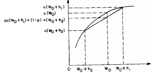
Figure: A strictly concave utility function — expected utility lies below utility of expected payoff
The above figure (conceptually) shows:
\[ u(W_0) > p \cdot u(W_0 + h_1) + (1 - p) \cdot u(W_0 + h_2) \]
The expected utility lies below the chord joining \( u(W_0 + h_1) \) and \( u(W_0 + h_2) \) — a hallmark of strict concavity. This visual demonstrates that the individual prefers the sure amount over the fair gamble, thus confirming strict risk aversion.
Portfolio Choice of a Risk-Averse Individual
Consider a risk-averse individual who has strictly increasing and concave utility over final wealth. They must allocate an initial wealth \( W_0 \) between a risk-free asset and a set of risky assets.
Let \( r_f \) denote the return on the risk-free asset, and let \( r_j \) be the (random) return on the \( j \)-th risky asset. Let \( \alpha_j \) denote the dollar amount invested in risky asset \( j \). The remaining wealth \( W_0 - \sum_j \alpha_j \) is invested in the risk-free asset.
The total wealth at the end of the period, \( W \), is then given by:
\[ W = (W_0 - \sum_j \alpha_j)(1 + r_f) + \sum_j \alpha_j (1 + r_j) \]Expanding and simplifying:
\[ W = W_0(1 + r_f) + \sum_j \alpha_j (r_j - r_f) \]The individual's objective is to choose the allocation \( \{\alpha_j\} \) to maximize expected utility of wealth:
\[ \max_{\{\alpha_j\}} \mathbb{E}\left[u\left(W_0(1 + r_f) + \sum_j \alpha_j (r_j - r_f)\right)\right] \]Since \( u \) is concave and differentiable, we can derive first-order conditions for optimality by differentiating the objective with respect to each \( \alpha_j \) and setting the derivative equal to zero:
\[ \frac{\partial}{\partial \alpha_j} \mathbb{E}[u(W)] = \mathbb{E}\left[u'(W)(r_j - r_f)\right] = 0 \quad \forall j \]These first-order conditions are necessary and sufficient due to concavity of \( u \). They imply that the marginal utility-weighted return in excess of the risk-free rate must be zero in expectation.
Finally, because \( u \) is strictly increasing, \( u'(W) > 0 \), so the expected excess returns \( r_j - r_f \) must take both positive and negative values. That is, the distribution of risky returns must be non-degenerate.
This framework is fundamental in modern portfolio theory, leading directly to concepts like the Capital Asset Pricing Model (CAPM) under additional assumptions.
Risk Aversion and Risky Investment
An individual who is risk averse and strictly prefers more to less (i.e., has a strictly increasing and concave utility function) will invest in risky assets if and only if at least one of those assets has a strictly positive risk premium.
Let the risk-free rate be denoted by \( r_f \), and let the random return of the \( j \)-th risky asset be \( r_j \). The individual's optimal allocation \( \alpha_j \) in the \( j \)-th risky asset satisfies the first-order condition:
\[ \mathbb{E}[u'(W)(r_j - r_f)] = 0 \quad \forall j \]Suppose the individual does not invest in any risky asset, i.e., \( \alpha_j = 0 \ \forall j \). Then their end-of-period wealth is risk-free: \( W = W_0(1 + r_f) \). Because \( u' > 0 \), the first-order condition at \( \alpha_j = 0 \) implies:
\[ \mathbb{E}[r_j - r_f] \leq 0 \quad \forall j \]That is, unless every risky asset has non-positive expected excess return, the individual has an incentive to take some positive risky position. Hence, the individual will avoid all risky investments only if:
\[ \mathbb{E}[r_j - r_f] \leq 0 \quad \forall j \]On the other hand, if there exists at least one risky asset \( j' \) such that:
\[ \mathbb{E}[r_{j'} - r_f] > 0 \]then there exists at least one risky asset \( j \) such that the individual will optimally allocate a positive amount to it:
\[ \exists j \text{ such that } \alpha_j > 0 \]Importantly, when multiple risky assets are available, the asset with the highest risk premium is not necessarily the one receiving a positive investment, due to diversification effects. However, when there is only one risky asset, this simplifies: a strictly positive risk premium directly implies a positive investment in that asset.
Minimum Risk Premium for Full Investment
We consider a strictly risk-averse individual who prefers more to less. The economy contains one risky asset and one risk-free asset. If the risky asset has a strictly positive risk premium, Section 1.19 ensures that the individual will make a strictly positive investment in it.
This section focuses on determining the minimum risk premium required to induce the individual to invest all of their wealth in the risky asset. Let \( i \) be the rate of return on the risky asset and \( r_f \) the risk-free rate. The investment decision must satisfy:
\[ \mathbb{E}\left[u'(W_0(1 + i))(i - r_f)\right] \geq 0 \]We take a first-order Taylor expansion of \( u'(W_0(1 + i)) \) around \( W_0(1 + r_f) \):
\[ u'(W_0(1 + i)) \approx u'(W_0(1 + r_f)) + u''(W_0(1 + r_f)) \cdot W_0(i - r_f) \]Multiplying both sides by \( (i - r_f) \) and taking expectations:
\[ \mathbb{E}[u'(W_0(1 + i)) \cdot (i - r_f)] \approx u'(W_0(1 + r_f)) \cdot \mathbb{E}[i - r_f] + u''(W_0(1 + r_f)) \cdot W_0 \cdot \mathbb{E}[(i - r_f)^2] \]To find the minimum risk premium required to induce full risky investment, we set the expression to zero:
\[ u'(W_0(1 + r_f)) \cdot \mathbb{E}[i - r_f] + u''(W_0(1 + r_f)) \cdot W_0 \cdot \mathbb{E}[(i - r_f)^2] = 0 \]Solving for the expected excess return \( \mathbb{E}[i - r_f] \), we get:
\[ \mathbb{E}[i - r_f] = -\frac{u''(W_0(1 + r_f))}{u'(W_0(1 + r_f))} \cdot W_0 \cdot \mathbb{E}[(i - r_f)^2] \]Using the Arrow-Pratt measure of absolute risk aversion, defined as
\[ R_A(x) = -\frac{u''(x)}{u'(x)}, \]we write the final expression as:
\[ \mathbb{E}[i - r_f] = R_A(W_0(1 + r_f)) \cdot W_0 \cdot \mathbb{E}[(i - r_f)^2] \]This measure is meaningful because it remains invariant under strictly positive affine transformations of the utility function (i.e., changes of the form \( au(x) + b \), with \( a > 0 \)). Hence, unlike the second derivative alone, it properly captures the curvature-related intensity of risk aversion in expected utility theory.
Absolute Risk Aversion and Behavior Toward Risky Assets
Absolute risk aversion, defined by the Arrow-Pratt measure as \[ R_A(z) = -\frac{u''(z)}{u'(z)}, \] characterizes how an individual's risk tolerance changes with wealth. Depending on how \( R_A(z) \) changes with \( z \), we classify preferences as:
- Decreasing Absolute Risk Aversion (DARA): \( \frac{dR_A(z)}{dz} < 0 \). The individual becomes more tolerant to risk as wealth increases.
- Increasing Absolute Risk Aversion (IARA): \( \frac{dR_A(z)}{dz} > 0 \). The individual becomes less tolerant to risk with more wealth.
- Constant Absolute Risk Aversion (CARA): \( \frac{dR_A(z)}{dz} = 0 \). Risk tolerance does not change with wealth.
Arrow (1970) showed the economic significance of these patterns. Suppose an individual chooses between a riskless asset and a single risky asset. Then:
- If the utility function exhibits DARA, the risky asset behaves like a normal good: demand for it increases with wealth.
- If the utility exhibits IARA, the risky asset is an inferior good: demand decreases as wealth increases.
- If CARA holds, demand is independent of wealth.
The goal is to determine how an individual’s optimal investment in the risky asset, denoted \( a \), changes with initial wealth \( W_0 \).
First-Order Condition
The first-order condition (FOC) for optimal investment is: \[ \mathbb{E}\left[ u'(W) \cdot (i - r_f) \right] = 0, \] where final wealth is \( W = W_0(1 + r_f) + a(i - r_f) \), and \( i \) is the random return on the risky asset.
How Optimal Investment Changes with Wealth
To study how \( a \) changes with \( W_0 \), we apply implicit differentiation to the FOC. Differentiating both sides with respect to \( W_0 \), we get: \[ \frac{da}{dW_0} = \frac{ \mathbb{E}\left[ u''(W)(i - r_f) \cdot (1 + r_f) \right] }{ \mathbb{E}\left[ u''(W)(i - r_f)^2 \right] }. \] This is equation (1.21.1).
Since \( u''(W) < 0 \), the denominator is negative. Therefore, the sign of \( \frac{da}{dW_0} \) depends on the sign of the numerator: \[ \text{sign} \left( \frac{da}{dW_0} \right) = \text{sign} \left( \mathbb{E}[u''(W)(i - r_f)] \right). \]
Role of Decreasing Absolute Risk Aversion
Under DARA, \( R_A(z) \) is strictly decreasing, i.e., \( \frac{dR_A(z)}{dz} < 0 \). Since wealth \( W \) depends positively on \( W_0 \), and the return \( i \) is uncertain, we split the expectation based on return cases:
- When \( i \geq r_f \), then \( W \geq W_0(1 + r_f) \), so DARA implies: \[ u''(W) > -R_A(W_0(1 + r_f)) \cdot u'(W) \]
- When \( i < r_f \), then \( W < W_0(1 + r_f) \), so DARA implies: \[ u''(W) < -R_A(W_0(1 + r_f)) \cdot u'(W) \]
Multiplying both cases by \( (i - r_f) \) and taking expectations across \( i \), and using the FOC \(\mathbb{E}[u'(W)(i - r_f)] = 0\), we find: \[ \mathbb{E}[u''(W)(i - r_f)] > 0 \Rightarrow \frac{da}{dW_0} > 0 \] This confirms that under DARA, investment in the risky asset increases with wealth.
Third Derivative and Risk Aversion Dynamics
Finally, the property \( \frac{dR_A(z)}{dz} < 0 \) implies the third derivative of utility is positive: \[ \frac{dR_A(z)}{dz} = \frac{ -u'''(z)u'(z) + [u''(z)]^2 }{ [u'(z)]^2 } \leq 0 \Rightarrow u'''(z) > 0 \] This tells us that for DARA behavior, the utility function is strictly increasing, concave, and its rate of concavity decreases—i.e., the individual becomes less risk averse as wealth grows.
Common Utility Functions and Risk Aversion Behavior
In finance, several standard utility functions are used to model risk aversion and its impact on investment decisions. These functions help determine whether the risky asset behaves like a normal or inferior good, and how investment demand changes with wealth.
1. Quadratic Utility Function
\[ u(z) = z - bz^2, \quad b > 0 \] First and second derivatives: \[ u'(z) = 1 - 2bz, \quad u''(z) = -2b \] Absolute risk aversion: \[ R_A(z) = \frac{-u''(z)}{u'(z)} = \frac{2b}{1 - 2bz} \] Its derivative: \[ \frac{dR_A(z)}{dz} = \frac{4b^2}{(1 - 2bz)^2} > 0 \] So, this utility function exhibits increasing absolute risk aversion (IARA). As wealth increases, the individual becomes more risk averse. Thus, the risky asset is considered an inferior good.
2. Negative Exponential Utility Function
\[ u(z) = -e^{-bz}, \quad b > 0 \] Derivatives: \[ u'(z) = be^{-bz} > 0, \quad u''(z) = -b^2e^{-bz} < 0 \] Absolute risk aversion: \[ R_A(z) = \frac{-u''(z)}{u'(z)} = b \quad \text{(constant)} \] So, \[ \frac{dR_A(z)}{dz} = 0 \] This function shows constant absolute risk aversion (CARA). The amount invested in the risky asset is independent of wealth. Any change in wealth is absorbed via the riskless asset.
3. Narrow Power Utility Function
\[ u(z) = \frac{z^{1 - B}}{1 - B}, \quad B > 0, z > 0 \] Derivatives: \[ u'(z) = z^{-B}, \quad u''(z) = -Bz^{-B - 1} \] Absolute and relative risk aversion: \[ R_A(z) = \frac{-u''(z)}{u'(z)} = \frac{B}{z}, \quad R_R(z) = z \cdot R_A(z) = B \] Derivatives: \[ \frac{dR_A(z)}{dz} = -\frac{B}{z^2} < 0, \quad \frac{dR_R(z)}{dz} = 0 \] So, this function exhibits decreasing absolute risk aversion (DARA) and constant relative risk aversion (CRRA). The proportion of wealth allocated to risky assets stays fixed as wealth changes.
4. Extended Power Utility Function
\[ u(z) = \frac{(A + Bz)^{1 - \gamma}}{1 - \gamma}, \quad B > 0,\ \gamma > 0,\ z > \max\left(0, -\frac{A}{B}\right) \] Derivatives: \[ u'(z) = B(A + Bz)^{-\gamma}, \quad u''(z) = -\gamma B^2(A + Bz)^{-\gamma - 1} \] Absolute and relative risk aversion: \[ R_A(z) = \frac{-u''(z)}{u'(z)} = \frac{\gamma B}{A + Bz}, \quad R_R(z) = z \cdot R_A(z) = \frac{\gamma B z}{A + Bz} \] Derivatives: \[ \frac{dR_A(z)}{dz} = -\frac{\gamma B^2}{(A + Bz)^2} < 0 \] \[ \frac{dR_R(z)}{dz} = \frac{\gamma B A}{(A + Bz)^2} \] Interpretation:
- If \( A > 0 \): \( \frac{dR_R(z)}{dz} > 0 \) ⇒ Increasing relative risk aversion (IRRA)
- If \( A = 0 \): \( \frac{dR_R(z)}{dz} = 0 \) ⇒ Constant relative risk aversion (CRRA)
- If \( A < 0 \): \( \frac{dR_R(z)}{dz} < 0 \) ⇒ Decreasing relative risk aversion (DRRA)
Exercises from Huang and Litzenberger
Exercise 1.1: Countable Set and Utility Representation
Let \( X \) be a countable set. A binary relation \( \succeq \) on \( X \) is a preference relation if and only if it can be represented by a real-valued function.
Intuitively, a preference relation expresses the idea that one element is at least as desirable as another. If such a relation exists on a countable set, it is always possible to assign real numbers (utilities) to the elements such that higher numbers represent more preferred elements.
For example, if you have a countable list of products (like coffee brands), you can rank them by assigning utilities: A = 3, B = 2, C = 1 to reflect preferences A ≻ B ≻ C. This ordinal utility captures the preference structure.
Proof: Suppose \( X = \{x_1, x_2, x_3, \ldots\} \) is countable. Define a function \( u: X \rightarrow \mathbb{R} \) such that for all \( x_i, x_j \in X \), \[ x_i \succeq x_j \iff u(x_i) \geq u(x_j). \] This is done by assigning numbers to each element respecting the preference order. Since the set is countable, we can construct such a function step-by-step.
Conversely, if a function \( u \) exists such that \( x \succeq y \iff u(x) \geq u(y) \), then the relation is complete and transitive by properties of real numbers. Thus, it is a preference relation.
Hence, a binary relation on a countable set is a preference relation if and only if it admits a utility representation.
Exercise 1.2: Lexicographic Preferences and Non-Representability
Define \( X = [0,1] \times [0,1] \) and the relation \( (x_1, x_2) \succeq (y_1, y_2) \) if either \( x_1 > y_1 \), or \( x_1 = y_1 \) and \( x_2 \geq y_2 \). This is known as the lexicographic preference relation.
1.2.1 Verification of Preference Relation
The relation is complete because for any two elements, one of the comparison conditions must hold. It is transitive because if \( x \succeq y \) and \( y \succeq z \), then either \( x_1 > y_1 \) or \( x_1 = y_1 \) and \( x_2 \geq y_2 \), and similarly for \( y \succeq z \). These conditions together imply \( x \succeq z \). Thus, the relation is a preference relation.
1.2.2 Strict Comparison Implies Equality
Suppose both \( x \succeq y \) and \( y \succeq x \). Then:
- If \( x_1 > y_1 \), then \( y \not\succeq x \)
- If \( x_1 = y_1 \) and \( x_2 > y_2 \), then again \( y \not\succeq x \)
- Only possibility for both to hold is when \( x_1 = y_1 \) and \( x_2 = y_2 \)
1.2.3 Non-Representability by Real-Valued Function
The representation theorem states that a binary relation \( \succeq \) can be represented by a real-valued function if it is a preference relation and there exists a countable \( \succeq \)-order dense subset \( Y \subset X \). We already verified \( \succeq \) is a preference relation.
Suppose \( Y \subset X \) is countable and order-dense. Pick two points \( x = (x_1, x_2) \) and \( x' = (x_1, x_2') \) with \( x_2 < x_2' \). Any point between them under the lexicographic relation must have the same first coordinate \( x_1 \) and second coordinate strictly between \( x_2 \) and \( x_2' \). But the interval \( (x_2, x_2') \) is uncountable, so no countable subset can intersect all such intervals. Therefore, no countable \( \succeq \)-order dense set exists.
Since one of the conditions of the representation theorem fails, this lexicographic preference relation cannot be represented by a real-valued utility function.
Problem 1.4
Part 1: Show that a von Neumann–Morgenstern (vNM) utility function is determined up to a strictly positive linear transformation.
✦ What is a von Neumann–Morgenstern utility function?
The vNM utility function assigns numbers to outcomes (lotteries or gambles) such that preferred lotteries have higher expected utility. Only the order of preference matters, not the actual utility numbers.
✦ What does "determined up to a strictly positive linear transformation" mean?
If \( u \) is a vNM utility function, then any function of the form:
\[ v(z) = a \cdot u(z) + b, \quad \text{where } a > 0 \]
represents the same preferences.
Proof Sketch:
Assume \( u \) represents preferences, so:
\[ p \succ q \iff \sum_z u(z)p(z) > \sum_z u(z)q(z) \]
Now define \( v(z) = a \cdot u(z) + b \). Then:
\[ \sum_z v(z)p(z) = a \sum_z u(z)p(z) + b \sum_z p(z) = a \sum_z u(z)p(z) + b \]
Since \( \sum_z p(z) = 1 \), the additive constant \( b \) does not affect preference. As \( a > 0 \), inequality direction is preserved.
Conclusion: \( v \) represents the same preference ordering as \( u \).
Part 2: Show that if a binary relation \( \succeq \) has an expected utility representation \( u \), then it satisfies the three vNM axioms.
✦ Recap of the Three vNM Axioms:
- Completeness & Transitivity: You can compare any two lotteries, and your preferences are logically consistent.
- Continuity: Preferences change smoothly; if \( A \succ B \succ C \), then some mix of \( A \) and \( C \) is equally preferred to \( B \).
- Independence: If \( A \succ B \), then for any third lottery \( C \), a mix with \( A \) is still preferred to a mix with \( B \).
Intuitive Justification:
Given:
\[ p \succeq q \iff \sum_z u(z)p(z) \geq \sum_z u(z)q(z) \]
- Completeness & Transitivity: Numbers can always be compared and maintain transitivity.
- Continuity: If \( u(p) > u(q) > u(r) \), then there exists a mix of \( p \) and \( r \) that equals \( u(q) \).
- Independence: Expected utility is linear in probabilities, so mixing with a third lottery preserves preference order.
Problem 1.5
Prove that:
\[ \frac{d R_A(z)}{dz} > 0 \Rightarrow \frac{d a}{dW_0} < 0 \quad \forall W_0 \]
and
\[ \frac{d R_A(z)}{dz} = 0 \Rightarrow \frac{d a}{dW_0} = 0 \quad \forall W_0 \]
✦ Arrow–Pratt Absolute Risk Aversion:
\[ R_A(z) = -\frac{u''(z)}{u'(z)} \]
Measures how risk averse a person is at wealth level \( z \).
✦ What is \( a \)?
It’s the optimal investment in a risky asset depending on initial wealth \( W_0 \).
Interpretation:
- If \( \frac{d R_A(z)}{dz} > 0 \), risk aversion increases with wealth. So, richer individuals invest less in risk: \( \frac{d a}{dW_0} < 0 \).
- If \( R_A(z) \) is constant, then \( a \) doesn't change with wealth: \( \frac{d a}{dW_0} = 0 \).
Real-Life Analogy:
Two people with ₹1 lakh. One becomes more conservative as wealth grows — reduces risky investment. The other stays consistent regardless of wealth.
Problem 1.6
Show that:
\[ \frac{d R_R(z)}{dz} < 0 \quad \forall z \in \mathbb{R} \Rightarrow \eta > 1 \]
\[ \frac{d R_R(z)}{dz} = 0 \quad \forall z \in \mathbb{R} \Rightarrow \eta = 1 \]
✦ Relative Risk Aversion:
\[ R_R(z) = - \frac{z \cdot u''(z)}{u'(z)} \]
✦ Wealth Elasticity of Demand:
\[ \eta = \frac{d \log a}{d \log W_0} = \frac{W_0}{a} \cdot \frac{d a}{d W_0} \]
Interpretation:
- If \( \frac{dR_R}{dz} < 0 \), you're more risk-tolerant when wealthier → demand grows faster than wealth → \( \eta > 1 \)
- If \( R_R(z) \) is constant, then risky investment scales linearly → \( \eta = 1 \)
Example:
- Person A triples risky investment when wealth doubles → \( \eta = 1.5 \)
- Person B doubles risky investment with doubling wealth → \( \eta = 1 \)
Summary Table
| Concept | Condition | Implication |
|---|---|---|
| vNM Utility | \( v = a u + b, a > 0 \) | Preference preserved |
| Expected utility exists | — | Satisfies vNM axioms |
| Increasing Absolute Risk Aversion | \( dR_A/dz > 0 \) | \( da/dW_0 < 0 \) |
| Constant Absolute Risk Aversion | \( dR_A/dz = 0 \) | \( da/dW_0 = 0 \) |
| Decreasing Relative Risk Aversion | \( dR_R/dz < 0 \) | \( \eta > 1 \) |
| Constant Relative Risk Aversion | \( dR_R/dz = 0 \) | \( \eta = 1 \) |
Problem Statement Recap
We are given:
- An individual with an increasing, strictly concave utility function \( u \).
- A fair gamble: gain \( h_1 \) with probability \( p \), loss \( h_2 \) with probability \( 1 - p \), with: \[ p h_1 + (1 - p) h_2 = 0 \]
- The insurance premium \( z \) is defined by: \[ u(W_0 - z) = p\,u(W_0 + h_1) + (1 - p)\,u(W_0 + h_2) \]
- Let \( RA(z) = -\frac{u''(z)}{u'(z)} \) be the Arrow-Pratt measure of absolute risk aversion.
What We’re Asked to Show
We are to analyze how \( RA(z) \) behaves with respect to changes in initial wealth \( W_0 \), via the function \( z(W_0) \). Specifically, show that when the risk is small:
\[ \frac{d\,RA(z)}{d\,z} \begin{cases} < 0 & \text{if } \frac{d\,z(W_0)}{d\,W_0} < 0 \\ = 0 & \text{if } \frac{d\,z(W_0)}{d\,W_0} = 0 \\ > 0 & \text{if } \frac{d\,z(W_0)}{d\,W_0} > 0 \end{cases} \]Solution (with Intuition and Derivation)
1. Setup
We define the premium \( z \) such that the expected utility of the gamble equals the utility of certainty:
\[ u(W_0 - z) = p\,u(W_0 + h_1) + (1 - p)\,u(W_0 + h_2) \]Since \( h_1, h_2 \) are small (small risk assumption), we can expand both sides using Taylor expansion around \( W_0 \).
2. First-Order Approximation (Taylor Expansion)
Left-hand side:
\[ u(W_0 - z) \approx u(W_0) - z u'(W_0) + \frac{z^2}{2} u''(W_0) \]Right-hand side:
\[ p u(W_0 + h_1) + (1 - p) u(W_0 + h_2) \approx u(W_0) + [p h_1 + (1 - p) h_2] u'(W_0) + \frac{1}{2} [p h_1^2 + (1 - p) h_2^2] u''(W_0) \]But since the gamble is fair:
\[ p h_1 + (1 - p) h_2 = 0 \]So the RHS becomes:
\[ u(W_0) + \frac{1}{2} \underbrace{[p h_1^2 + (1 - p) h_2^2]}_{=: \sigma^2} u''(W_0) \]Now equate both sides:
\[ u(W_0) - z u'(W_0) + \frac{1}{2} z^2 u''(W_0) = u(W_0) + \frac{1}{2} \sigma^2 u''(W_0) \]Subtract \( u(W_0) \) from both sides:
\[ - z u'(W_0) + \frac{1}{2} z^2 u''(W_0) = \frac{1}{2} \sigma^2 u''(W_0) \]Multiply both sides by 2:
\[ -2 z u'(W_0) + z^2 u''(W_0) = \sigma^2 u''(W_0) \]Rearrange:
\[ z^2 u''(W_0) - 2 z u'(W_0) - \sigma^2 u''(W_0) = 0 \]This is a quadratic in \( z \). Solve for \( z \):
\[ z = \frac{2 u'(W_0) \pm \sqrt{4 u'(W_0)^2 + 4 u''(W_0)^2 \sigma^2}}{2 u''(W_0)} \]Ignore the + root (negative premium not meaningful), and simplify for small \( \sigma \):
\[ z \approx \frac{\sigma^2}{2} \cdot \left( - \frac{u''(W_0)}{u'(W_0)} \right) = \frac{\sigma^2}{2} \cdot RA(W_0) \]So we have:
\[ z(W_0) \approx \frac{\sigma^2}{2} RA(W_0) \]This tells us:
- The premium \( z \) is proportional to the Arrow–Pratt risk aversion measure.
3. Differentiate \( RA(z) \) w.r.t \( z \)
Now, \( RA(z) = -\frac{u''(z)}{u'(z)} \), and \( z = z(W_0) \).
Differentiate \( RA(z) \) w.r.t \( W_0 \):
\[ \frac{d\,RA(z)}{d\,W_0} = \frac{d\,RA(z)}{dz} \cdot \frac{dz}{dW_0} \]So:
- If \( \frac{dz}{dW_0} > 0 \), then \( \frac{d\,RA(z)}{d\,W_0} \) has the same sign as \( \frac{d\,RA(z)}{dz} \)
- If \( \frac{dz}{dW_0} < 0 \), then it has the opposite sign
Hence, the sign of \( \frac{d\,RA(z)}{dz} \) is determined by the sign of \( \frac{dz}{dW_0} \):
\[ \frac{d\,RA(z)}{dz} \begin{cases} < 0 & \text{if } \frac{dz}{dW_0} < 0 \\ = 0 & \text{if } \frac{dz}{dW_0} = 0 \\ > 0 & \text{if } \frac{dz}{dW_0} > 0 \end{cases} \]Final Answer
So when the risk is small (i.e., \( h_1, h_2 \) are small), we have:
\[ \frac{d\,RA(z)}{dz} \begin{cases} < 0 & \text{if } \frac{dz(W_0)}{dW_0} < 0 \\ = 0 & \text{if } \frac{dz(W_0)}{dW_0} = 0 \\ > 0 & \text{if } \frac{dz(W_0)}{dW_0} > 0 \end{cases} \]Last updated: July 17, 2025