1. Definition
A Markov process \(X_t\) is a stochastic process with the property that, given the value of \(X_t\), the values of \(X_s\) for s>t are not influenced by the values of \(X_u\) for \(t> u\).
A discrete-time Markov chain is a Markov process whose state space is a finite or countable set, and whose (time) index set is T =\( (0,1,2 \ldots ) \). Mathematically: $$ P(X_{n+1} = j| X_0 = i_0, \ldots , X_{n-1} = i_{n-1}, X_n= i) $$ $$ = P( X_{n+1} =j | X_n= i) $$ for all n and all states \( i_0 , \ldots, i_{n-1}, i, j \)
Understanding One-Step Transition Probabilities
In a Markov chain, we usually label the state space using non-negative integers: 0, 1, 2, .... Unless stated otherwise, we follow this convention.
If the chain is in a certain state at time \( n \), we say \( X_n = i \). The probability that it moves to state \( j \) at the next time step \( n+1 \), given that it is currently in state \( i \), is called the one-step transition probability. It is denoted by:
\[ P^{(n,n+1)}_{ij} = \Pr(X_{n+1} = j \mid X_n = i) \]This notation indicates that the transition probabilities can depend on the current time \( n \), as well as the current and next states \( i \) and \( j \).
If these probabilities are independent of time, we say that the Markov chain has stationary transition probabilities. In that case, we write:
\[ P_{ij} = \Pr(X_{n+1} = j \mid X_n = i) \]This means the probability of transitioning from state \( i \) to state \( j \) remains the same at every step.
These probabilities \( P_{ij} \) are usually arranged in a transition matrix \( P \) as follows:
\[ P = \begin{bmatrix} P_{00} & P_{01} & P_{02} & \cdots \\ P_{10} & P_{11} & P_{12} & \cdots \\ P_{20} & P_{21} & P_{22} & \cdots \\ \vdots & \vdots & \vdots & \ddots \\ \end{bmatrix} \]Each row corresponds to the current state \( i \), and each column represents the probability of transitioning to state \( j \).
The Markov Transition Matrix
In a Markov chain, we represent the one-step transition probabilities using a matrix \( P \), called the Markov matrix or transition probability matrix. Each entry \( P_{ij} \) in this matrix represents the probability of moving from state \( i \) to state \( j \) in one step.
That is, \[ P_{ij} = \Pr(X_{n+1} = j \mid X_n = i) \]
The \( i \)th row of \( P \) gives the full probability distribution of the next state \( X_{n+1} \) given that the current state \( X_n = i \). In other words, the \( i \)th row shows where the process might go from state \( i \), and with what probabilities.
If the number of states is finite (say, \( 0, 1, \ldots, r \)), then \( P \) is a finite square matrix of order \( r + 1 \), meaning it has \( r+1 \) rows and \( r+1 \) columns.
Conditions for Valid Transition Matrices
The entries of the transition matrix must satisfy two conditions:
- Non-negativity: All entries must be non-negative: \[ P_{ij} \geq 0 \quad \text{for all } i, j \]
- Row sums equal to 1: The probabilities in each row must sum to 1: \[ \sum_{j=0}^{r} P_{ij} = 1 \quad \text{for all } i \]
The second condition simply reflects the fact that some transition must occur at each step. Even if the state doesn't change (i.e., it stays in the same state), we still consider that a transition has occurred.
Theorem: A Markov process is completely defined once we specify its Markov matrix P and its initial state \( X_0 \)
Let P{ \( X_0 = i \)} = \(p_{i_0}\). It's enough to show how to compute the probability P{ \( X_0 = i_0, X_1 =i_1, \ldots , X_n= i_n \) }, since any probability containing \(X_{j_1}, X_{j_2}, \ldots, X_{j_k} , j_k> \ldots >j_2 >j_1 \) can be obtained by summing terms of the above form (by Theorem of Total Probability).
P{ \( X_0 = i_0, X_1 =i_1, \ldots , X_n= i_n \) }
=P{ \( X_0 = i_0, X_1 =i_1, \ldots , X_{n-1}= i_{n-1} \) } P{ \(X_n = i_n | X_0 = i_0, X_1 =i_1, \ldots , X_{n-1}= i_{n-1} \) }
=P{ \( X_0 = i_0, X_1 =i_1, \ldots , X_{n-1}= i_{n-1} \) } P{ \(X_n = i_n | X_{n-1}=i_{n-1} \) }
=P{ \( X_0 = i_0, X_1 =i_1, \ldots , X_{n-1}= i_{n-1} \) } \(P_{i_{n-1}i_n}\)
Similarly, P{ \( X_0 = i_0, X_1 =i_1, \ldots , X_n= i_{n-1} \) }
=P{ \( X_0 = i_0, X_1 =i_1, \ldots , X_{n-2}= i_{n-2} \) } \(P_{i_{n-2}i_{n-1}}\)
Therefore, the original expression simplifies to:
\( P\left( X_0 = i_0, X_1 = i_1, \ldots , X_n = i_n \right) = p_{i_0} \cdot P_{i_0 i_1} \cdot P_{i_1 i_2} \cdot \ldots \cdot P_{i_{n-1} i_n} \)
2 Transition Probability Matrices of a Markov Chain: Understanding Multi-Step Transition Probabilities
A Markov chain is fully defined by two things:
- Its one-step transition probability matrix \( P \)
- Its initial state distribution (i.e., the probabilities of starting in each state)
Most of the analysis of Markov chains revolves around calculating the probabilities of different outcomes after several steps or time periods. For this, we use the n-step transition probability matrix, denoted by \( P^{(n)} \).
The element \( P^{(n)}_{ij} \) represents the probability that the process moves from state \( i \) to state \( j \) in exactly \( n \) steps. Formally:
\( P^{(n)}_{ij} = \Pr(X_{m+n} = j \mid X_m = i) \)
Since we are considering stationary (time-homogeneous) Markov chains, the probability depends only on the number of steps \( n \), and not on the starting time \( m \).
Thanks to the Markov property (which says that the future depends only on the present state, not the past), we can compute \( P^{(n)} \) recursively:
\( P^{(n)}_{ij} = \sum_{k=0}^{\infty} P_{ik} \cdot P^{(n-1)}_{kj} \)
This recursive formula is just standard matrix multiplication, so we can write:
\( P^{(n)} = P \cdot P^{(n-1)} \)
By repeatedly applying this formula (i.e., multiplying the matrix \( P \) with itself \( n \) times), we get:
\( P^{(n)} = P^n \)
That is, the n-step transition probabilities are exactly the entries of the matrix \( P \) raised to the \( n \)-th power.
To complete the definition, we also define:
- \( P^{(0)}_{ij} = 1 \) if \( i = j \)
- \( P^{(0)}_{ij} = 0 \) if \( i \neq j \)
This just means that in zero steps, the process stays where it is.
Proof of the n-Step Transition Probability Formula
We want to prove the formula:
\( P^{(n)}_{ij} = \sum_{k} P_{ik} \cdot P^{(n-1)}_{kj} \)
This formula means: the probability of going from state \( i \) to state \( j \) in \( n \) steps is the sum over all intermediate states \( k \) of the probability of:
- Going from \( i \) to \( k \) in one step: \( P_{ik} \), and
- Then from \( k \) to \( j \) in \( n-1 \) steps: \( P^{(n-1)}_{kj} \)
To see why this works, let’s look at what it means to reach \( j \) from \( i \) in exactly \( n \) steps.
We imagine that the first step takes the process from state \( i \) to some state \( k \). Then the remaining \( n - 1 \) steps must take the process from \( k \) to \( j \).
Now, because of the Markov property, once the process reaches \( k \), it "forgets" how it got there. So the probability of continuing from \( k \) to \( j \) depends only on \( k \), and not on any earlier states.
So, for each possible intermediate state \( k \), the probability of going from \( i \rightarrow k \rightarrow j \) in total \( n \) steps is:
\( \Pr(X_1 = k \mid X_0 = i) \cdot \Pr(X_n = j \mid X_1 = k) = P_{ik} \cdot P^{(n-1)}_{kj} \)
To find the total probability of reaching \( j \) from \( i \) in \( n \) steps, we sum this product over all possible intermediate states \( k \):
\( P^{(n)}_{ij} = \sum_{k} P_{ik} \cdot P^{(n-1)}_{kj} \)
This is exactly how matrix multiplication works, so we can write the matrix formula:
\( P^{(n)} = P \cdot P^{(n-1)} \)
By repeating this step, we get:
\( P^{(n)} = P^n \)
This completes the proof. It uses the basic idea that the path from \( i \) to \( j \) in \( n \) steps must go through some state \( k \) after the first step, and the rest follows by the Markov property and total probability.
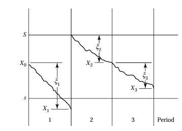
3(a). Inventory Model Using Markov Chains
This model describes a scenario where a commodity is stocked to meet a random demand over time. Time is divided into periods (n = 0, 1, 2, ...), and stock is reviewed at the end of each period.
The demand in each period, denoted by \( \xi_n \), is a random variable with the same probability distribution across time:
- \( \Pr(\xi_n = 0) = a_0 \)
- \( \Pr(\xi_n = 1) = a_1 \)
- \( \Pr(\xi_n = 2) = a_2 \)
- ... and so on, where \( \sum a_k = 1 \)
The stock is restocked based on the following policy:
- If the current stock is \( \leq s \), restock up to \( S \)
- If the stock is more than \( s \), no replenishment occurs
The state of the process is \( X_n \), the stock level at the end of period \( n \), before restocking. It evolves as a Markov chain based on the random demand and the restocking rule.
The transition rule is:
- If \( X_n > s \), then \( X_{n+1} = X_n - \xi_{n+1} \)
- If \( X_n \leq s \), then \( X_{n+1} = S - \xi_{n+1} \)
This rule, together with the demand probabilities, determines the transition probability matrix.
Example
Suppose:
- \( S = 2 \), \( s = 0 \)
- \( \Pr(\xi = 0) = 0.5 \), \( \Pr(\xi = 1) = 0.4 \), \( \Pr(\xi = 2) = 0.1 \)
Possible stock levels: 2, 1, 0, -1 (unfilled demand is treated as negative stock).
From this setup, we compute the transition probabilities. For instance:
- If \( X_n = 1 \), no restocking. To reach \( X_{n+1} = 0 \), \( \xi_{n+1} = 1 \). So \( P_{10} = 0.4 \)
- If \( X_n = 0 \), restock to 2. To reach \( X_{n+1} = 0 \), \( \xi_{n+1} = 2 \). So \( P_{00} = 0.1 \)
Transition Matrix:
       |  -1   0    1    2
    ------------------------
    -1 |  0   0.1  0.4  0.5
     0 |  0   0.1  0.4  0.5
     1 | 0.1  0.4  0.5   0
     2 |  0   0.1  0.4  0.5
Important Quantities
- Long-term probability of unfilled demand: \( \lim_{n \to \infty} \Pr(X_n < 0) \)
- Average inventory level: \( \lim_{n \to \infty} \sum_{j>0} j \cdot \Pr(X_n = j) \)
Visual Representation
Below is the illustration of how the process evolves over time:
3(b).Ehrenfest Urn Model
The Ehrenfest urn model is a classical representation of diffusion, simulating how molecules move across a membrane.
Imagine you have two containers (urns), A and B, that together contain a total of 2a balls. Initially, urn A holds k balls and urn B has 2a - k balls.
At each time step, one of the 2a balls is selected at random, and then moved to the other urn. This random movement simulates the diffusion of molecules.
Let Yn be the number of balls in urn A after the nth step, and define a centered variable:
Xn = Yn - a
Then Xn becomes a Markov chain with state space:
{ -a, -a+1, ..., 0, ..., a-1, a }
Transition Probabilities
The transition probabilities are defined as follows:
- \( P_{i,i+1} = \frac{a - i}{2a} \) (gain a ball in urn A)
- \( P_{i,i-1} = \frac{a + i}{2a} \) (lose a ball from urn A)
- All other transitions have zero probability.
This transition rule reflects that if urn A has more balls (i is positive), then it's more likely to lose a ball, and vice versa. Thus, there is a tendency or "drift" toward balancing the urns.
Equilibrium Distribution
An important focus of this model is finding the equilibrium distribution — the long-run behavior of the number of balls in urn A. Over time, the system stabilizes such that the probability distribution over states no longer changes.
The model is symmetric and reversible, so the equilibrium distribution exists and reflects the binomial distribution of balls across urn A and B, due to random uniform selection.
3(c). Markov Chains in Genetics
1. Simple Haploid Model (No Mutation or Selection)
This model investigates how gene frequencies fluctuate across generations. We assume:
- There are 2N haploid genes in each generation (e.g., from 2N bacteria).
- Each gene is either of type a or A.
- If there are j a-genes in the current generation, then the probability of picking an a-gene to pass on is:
pj = j / (2N), and qj = 1 − pj. - The next generation is formed by independently selecting 2N genes with replacement, using the above probabilities.
So, the number of a-genes in the next generation follows a Binomial(2N, pj) distribution.
We define a Markov chain Xn to be the number of a-genes in generation n. The state space is {0, 1, ..., 2N}.
Transition Probability:
The transition probability from state j to state k is:
Pjk = C(2N, k) * (pj)k * (qj)2N−k
where C(2N, k) = 2N choose k.
Fixation States:
- State 0 (all A) and state 2N (all a) are absorbing.
- Once the population hits either of these, it stays there forever (no variation left).
2. Adding Mutation
Now suppose each gene may mutate before reproduction:
- a → A with probability μ
- A → a with probability ν
Modified Probability of a-gene after Mutation:
Let j be the number of a-genes initially. After mutation, the expected number of a-genes becomes:
- Each of the j a-genes mutates to A with probability μ → contributes j(1 − μ) a-genes.
- Each of the (2N − j) A-genes mutates to a with probability ν → contributes (2N − j)ν a-genes.
Total expected number of a-genes after mutation = j(1 − μ) + (2N − j)ν
So, the probability that a randomly selected gene after mutation is an a-gene is:
pj = [j(1 − μ) + (2N − j)ν] / (2N)
And qj = 1 − pj
Consequences:
- Now, even if all genes are of one type, mutation allows the other type to reappear.
- Fixation does not occur. Instead, the chain converges to a steady-state distribution over the state space {0, ..., 2N}.
3. Adding Selection
To model natural selection, we suppose that a-genes have a reproductive advantage.
If a-genes have a selective advantage s, then:
- Each a-gene reproduces with probability proportional to (1 + s)
- Each A-gene reproduces with probability proportional to 1
Adjusted Probability of Choosing a-gene:
If there are j a-genes and (2N − j) A-genes, then total fitness = (1 + s)j + (2N − j)
So,
pj = [(1 + s)j] / [(1 + s)j + (2N − j)],
qj = 1 − pj
Biological Meaning:
- If s > 0, then a-genes are more likely to be passed on.
- The population will tend to drift toward all a-genes (state 2N), even if started with a mix.
- This models directional selection.
3(d). Discrete Queueing Markov Chain
1. System Overview
This is a model of a queueing system where:
- Customers arrive randomly during each time period.
- At most one customer is served in each period (if someone is present).
- If the queue is empty, no service occurs in that period.
A real-world example: A taxi stand where taxis arrive at fixed intervals. If no passengers are waiting, the taxi leaves immediately.
2. Customer Arrival Process
Let An be the number of new customers arriving in period n.
- The number of arrivals follows a probability distribution:
Pr(An = k) = ak, for k = 0, 1, 2, ... - The arrivals in each period are independent and identically distributed (i.i.d.).
- The probabilities satisfy:
Σ ak = 1, and ak ≥ 0.
3. State of the System
Define Xn as the number of customers in the queue at the start of period n.
During a period:
- If Xn ≥ 1: One customer is served, and An customers arrive.
- If Xn = 0: No service happens, but still An customers may arrive.
Update Rule:
The number of customers at the start of next period is:
Xn+1 = max(0, Xn − 1) + An
This captures the logic: one customer leaves (if present), and An arrive.
4. Transition Probability Matrix
Let’s denote the transition probability Pij = Pr(Xn+1 = j | Xn = i)
If i = 0 (no one is in queue):
- No one is served, so the new state is just An.
- P0k = ak
If i ≥ 1 (at least one customer in queue):
- One customer is served, so current queue becomes (i − 1).
- An new arrivals → New state = i − 1 + An
- Pij = aj − (i − 1), only if j ≥ i − 1
Example Matrix:
| From/To | 0 | 1 | 2 | 3 | 4 |
|---|---|---|---|---|---|
| 0 | a0 | a1 | a2 | a3 | a4 |
| 1 | 0 | a0 | a1 | a2 | a3 |
| 2 | 0 | 0 | a0 | a1 | a2 |
| 3 | 0 | 0 | 0 | a0 | a1 |
5. Long-term Behavior
Expected Number of Arrivals:
Let the expected number of new customers in a period be:
λ = Σ k * ak
Case 1: λ < 1 (stable system)
- Queue reaches a statistical equilibrium.
- A limiting distribution π = {πk} exists such that:
limn→∞ Pr(Xn = k | X0 = j) = πk
Case 2: λ ≥ 1 (unstable system)
- The queue size increases indefinitely over time.
- No steady-state distribution exists.
6. Important Metrics
1. Long-run Idle Time:
The system is idle (no customer) only in state 0.
Fraction of time idle = π0
2. Mean Number of Customers in System:
L = Σ (k * πk)
3. Long-run Mean Time a Customer Spends in the System (Little’s Law):
Let T be the expected time spent in system.
T = L / λ, where λ is the arrival rate
4 First Step Analysis
A surprising number of problems involving Markov chains can be solved using a technique called first step analysis. This technique works by analyzing what happens during the first step (or transition) of the Markov process and then using the law of total probability and the Markov property to build equations that involve unknown quantities of interest.
4.1 Simple First Step Analyses
Consider a Markov chain with three states: 0, 1, and 2. The transition probability matrix is structured as follows:
- From state 0: it always stays in state 0 (absorbing)
- From state 1: with probability α, it moves to state 0; with probability β, it stays in state 1; and with probability γ, it moves to state 2
- From state 2: it always stays in state 2 (absorbing)
Here, α + β + γ = 1, and α, β, γ are all greater than 0.
So, if the chain starts in state 1, it may stay there for a while but will eventually get absorbed into either state 0 or state 2.
There are two natural questions to ask:
- What is the probability that the process eventually ends up in state 0 (instead of 2)?
- How long, on average, does it take for the process to get absorbed into either state 0 or state 2?
To answer these questions, we use first step analysis.
Defining Variables
Let T be the time (step number) when the process is absorbed (enters state 0 or 2 for the first time).
Let u be the probability that the process is eventually absorbed in state 0, given it starts in state 1:
u = P[X_T = 0 | X_0 = 1]
Let v be the expected number of steps until absorption, again given that the process starts in state 1:
v = E[T | X_0 = 1]
Using First Step Analysis to Compute u
We break the analysis based on where the process goes in its first step from state 1:
- If it moves to state 0 (probability α), then T = 1 and X_T = 0
- If it moves to state 2 (probability γ), then T = 1 and X_T = 2
- If it stays in state 1 (probability β), the situation is the same as before — the process restarts from state 1
So the probability of eventually reaching state 0 from state 1, denoted u, satisfies:
u = α × 1 + β × u + γ × 0
Simplifying:
u = α + βu
Solving for u:
u - βu = α → u(1 - β) = α → u = α / (1 - β)
This quantity represents the conditional probability of eventual absorption into state 0, assuming the process starts in state 1.
Using First Step Analysis to Compute v
Now, we calculate v, the expected number of steps until absorption.
Again we break into cases:
- If the process moves to state 0 or 2 (probability α + γ), it takes exactly 1 step
- If it stays in state 1 (probability β), then it takes 1 step now, and on average another v steps in the future (since it returns to where it started)
So:
v = α × 1 + β × (1 + v) + γ × 1
v = (α + γ) × 1 + β(1 + v)
v = (1 - β) + β(1 + v)
Simplify:
v = 1 + βv → v(1 - β) = 1 → v = 1 / (1 - β)
Verification via Geometric Distribution
The absorption time T, starting from state 1, actually follows a geometric distribution:
P[T > k | X_0 = 1] = β^k for k = 0, 1, 2, ...
This means:
E[T | X_0 = 1] = ∑ (from k = 0 to ∞) β^k = 1 / (1 - β)
This matches the result we obtained from first step analysis. In this simple case, the result can be verified directly, but for more complex Markov chains, first step analysis is often the only feasible method.
Extension to a Four-State Markov Chain
Now we consider a more complex situation: a four-state Markov chain with states 0, 1, 2, and 3. The transition matrix is given by:
- State 0 and State 3 are absorbing states (once the process enters them, it stays there forever).
- States 1 and 2 are transient states (the process can leave them).
The general form of the transition matrix is:
    0   1   2   3
0 [ 1   0   0   0 ]
1 [P10 P11 P12 P13]
2 [P20 P21 P22 P23]
3 [ 0   0   0   1 ]
Because absorption occurs in state 0 or 3, and the initial state could be either 1 or 2 (both transient), the probability of absorption in state 0 depends on where the process starts. To address this, we define the following:
- T = first time the process reaches either state 0 or 3
- ui = probability that the process is absorbed in state 0, given that it started in state i (i = 1, 2)
- vi = expected time until absorption, given that it started in state i (i = 1, 2)
We also define for consistency:
- u0 = 1 (since it is already in state 0)
- u3 = 0 (since it's already in state 3 and never goes to 0)
- v0 = 0 and v3 = 0 (already absorbed)
First Step Analysis for u1 and u2
Suppose the process starts in state 1. The first step could result in:
- Moving to state 0: contributes P10 × 1
- Moving to state 1: contributes P11 × u1 (we're back where we started)
- Moving to state 2: contributes P12 × u2
This leads to the equation:
u1 = P10 + P11 × u1 + P12 × u2 (Equation 3.21)
Similarly, for state 2:
u2 = P20 + P21 × u1 + P22 × u2 (Equation 3.22)
These two equations can be solved simultaneously to find the values of u1 and u2.
Numerical Example
Consider the specific transition matrix:
    0    1    2    3
0 [ 1    0    0    0 ]
1 [0.4  0.3  0.2  0.1]
2 [0.1  0.3  0.3  0.3]
3 [0    0    0    1 ]
Substituting into the equations for u1 and u2:
u1 = 0.4 + 0.3 × u1 + 0.2 × u2
u2 = 0.1 + 0.3 × u1 + 0.3 × u2
Solving the system:
0.7u1 + 0.2u2 = 0.4
0.3u1 + 0.7u2 = 0.1
The solution is:
- u1 = 30/43
- u2 = 19/43
So, starting from state 2, the probability that the process is eventually absorbed in state 0 is 19/43, and in state 3 is 24/43 (since the total must sum to 1).
Mean Time to Absorption (v1, v2)
We now use first step analysis to find the expected number of steps until absorption, starting from state 1 or 2.
If we start from state 1:
- With probability P11, it returns to state 1 → additional v1 steps expected
- With probability P12, it goes to state 2 → additional v2 steps expected
The equation becomes:
v1 = 1 + P11 × v1 + P12 × v2
Similarly, for state 2:
v2 = 1 + P21 × v1 + P22 × v2
Substituting the numerical values:
v1 = 1 + 0.3 × v1 + 0.2 × v2
v2 = 1 + 0.3 × v1 + 0.3 × v2
Solving these:
0.7v1 - 0.2v2 = 1
-0.3v1 + 0.7v2 = 1
The solutions are:
- v1 = (90/43) ≈ 2.09
- v2 = (100/43) ≈ 2.33
Therefore, if the process starts from state 2, it will take about 2.33 steps, on average, before it gets absorbed into either state 0 or 3.
4.2 General Structure of Absorbing Markov Chains
Consider a finite-state Markov chain \( \{X_n\} \) with state space labeled \( 0, 1, \ldots, N \). Assume states \( 0, 1, \ldots, r-1 \) are transient, and states \( r, r+1, \ldots, N \) are absorbing.
The transition matrix \( P \) has the following block form:
\[ P = \begin{bmatrix} Q & R \\ 0 & I \end{bmatrix} \]Here, \( Q \) governs transitions among transient states, \( R \) represents transitions from transient to absorbing states, \( 0 \) is a zero matrix, and \( I \) is the identity matrix for absorbing states.
Probability of Absorption in a Given State
Let \( u_i^{(k)} = \mathbb{P}( \text{absorption in state } k \mid X_0 = i ) \), for \( i < r \), where \( k \geq r \) is a fixed absorbing state. A first-step analysis gives:
\[ u_i^{(k)} = P_{ik} + \sum_{j=0}^{r-1} P_{ij} u_j^{(k)} \]This yields a system of linear equations for \( u_0^{(k)}, u_1^{(k)}, \ldots, u_{r-1}^{(k)} \).
Example: A Rat in a Maze
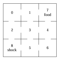
A rat moves randomly through a maze of 9 compartments. Compartments 7 (food) and 8 (shock) are absorbing. The transition probabilities are determined by uniform movement to adjacent compartments. Let \( u_i \) denote the probability that the rat reaches food (state 7) before shock (state 8), given that it starts at state \( i \).
Using first-step analysis, the equations are:
\[ \begin{aligned} u_0 &= \frac{1}{2}u_1 + \frac{1}{2}u_2 \\ u_1 &= \frac{1}{3}u_0 + \frac{1}{3}u_3 + \frac{1}{3} \\ u_2 &= \frac{1}{3}u_0 + \frac{1}{3}u_3 \\ u_3 &= \frac{1}{4}u_1 + \frac{1}{4}u_2 + \frac{1}{4}u_4 + \frac{1}{4}u_5 \\ u_4 &= \frac{1}{3}u_3 + \frac{1}{3}u_6 \\ u_5 &= \frac{1}{3}u_3 + \frac{1}{3}u_6 \\ u_6 &= \frac{1}{2}u_4 + \frac{1}{2}u_5 \\ u_7 &= 1 \\ u_8 &= 0 \end{aligned} \]By symmetry:
- \( u_0 = u_6 \)
- \( u_1 = u_4 \)
- \( u_2 = u_5 \)
- \( u_3 = \frac{1}{2} \)
This simplifies the system to:
\[ \begin{aligned} u_0 &= \frac{1}{2}u_1 + \frac{1}{2}u_2 \\ u_1 &= \frac{1}{3}u_0 + \frac{1}{3} \cdot \frac{1}{2} + \frac{1}{3} \\ u_2 &= \frac{1}{3}u_0 + \frac{1}{3} \cdot \frac{1}{2} \end{aligned} \]Solving these gives:
- \( u_0 = \frac{1}{2} \)
- \( u_1 = \frac{2}{3} \)
- \( u_2 = \frac{1}{3} \)
Expected Time Until Absorption
Define the absorption time:
\[ T = \min \{ n \geq 0 \mid X_n \geq r \} \]Let each transient state \( i \) have an associated rate \( g(i) \). Define:
\[ w_i = \mathbb{E} \left[ \sum_{n=0}^{T-1} g(X_n) \mid X_0 = i \right] \]This satisfies the equation:
\[ w_i = g(i) + \sum_{j=0}^{r-1} P_{ij} w_j \]Special Case 1: Mean Time to Absorption
If \( g(i) = 1 \) for all \( i \), then:
\[ v_i = \mathbb{E}[T \mid X_0 = i] = 1 + \sum_{j=0}^{r-1} P_{ij} v_j \]Special Case 2: Expected Visits to State \( k \)
If \( g(i) = \delta_{ik} \), then:
\[ W_{ik} = \mathbb{E}[\text{number of visits to } k \mid X_0 = i] = \delta_{ik} + \sum_{j=0}^{r-1} P_{ij} W_{jk} \]5 Some Special Markov Chains
We introduce several particular Markov chains that arise in a variety of applications.
5.1 The Two-State Markov Chain
Let the transition matrix be given by:
\[ P = \begin{bmatrix} 1 - a & a \\ b & 1 - b \end{bmatrix} \quad \text{where } 0 < a, b < 1 \tag{3.30} \]When \( a = 1 - b \), so that the rows of \( P \) are the same, then the states \( X_1, X_2, \dots \) are independent identically distributed (i.i.d.) random variables with \( \Pr(X_n = 0) = b \) and \( \Pr(X_n = 1) = a \). When \( a \ne 1 - b \), the probability distribution for \( X_n \) depends on the outcome \( X_{n-1} \) at the previous stage.
For the two-state Markov chain, it can be verified by induction that the n-step transition matrix is given by:
\[ P^n = \frac{1}{a + b} \left( \begin{bmatrix} b & a \\ b & a \end{bmatrix} + (1 - a - b)^n \begin{bmatrix} a & -a \\ -b & b \end{bmatrix} \right) \tag{3.31} \]To verify this formula, define the matrices:
\[ A = \begin{bmatrix} b & a \\ b & a \end{bmatrix}, \quad B = \begin{bmatrix} a & -a \\ -b & b \end{bmatrix} \]Then equation (3.31) becomes:
\[ P^n = \frac{1}{a + b} \left( A + (1 - a - b)^n B \right) \]Now check the matrix multiplications:
\[ AP = \begin{bmatrix} b & a \\ b & a \end{bmatrix} \begin{bmatrix} 1 - a & a \\ b & 1 - b \end{bmatrix} = \begin{bmatrix} b & a \\ b & a \end{bmatrix} = A \] \[ BP = \begin{bmatrix} a & -a \\ -b & b \end{bmatrix} \begin{bmatrix} 1 - a & a \\ b & 1 - b \end{bmatrix} = (1 - a - b) B \]Hence, for \( n = 1 \), we have:
\[ P^1 = \frac{1}{a + b} \left( A + (1 - a - b) B \right) = P \]To complete the induction, assume the formula holds for \( n \). Then:
\[ P^{n+1} = P^n P = \frac{1}{a + b} \left( A + (1 - a - b)^n B \right) P = \frac{1}{a + b} \left( A + (1 - a - b)^{n+1} B \right) \]This confirms the inductive step. Since \( 0 < a + b < 1 \), it follows that \( (1 - a - b)^n \to 0 \) as \( n \to \infty \), and thus:
\[ \lim_{n \to \infty} P^n = \frac{1}{a + b} \begin{bmatrix} b & a \\ b & a \end{bmatrix} \]Numerical Example
Suppose the items produced by a certain worker are graded as defective or not. Due to trends in raw material quality, whether or not a particular item is defective depends in part on whether or not the previous item was defective. Let \( X_n \) denote the quality of the \( n \)th item, with \( X_n = 0 \) meaning "good" and \( X_n = 1 \) meaning "defective."
Suppose \( X_n \) evolves as a Markov chain whose transition matrix is:
\[ P = \begin{bmatrix} 0.99 & 0.01 \\ 0.12 & 0.88 \end{bmatrix} \]Defective items tend to appear in bunches in the output of such a system. In the long run, the probability that an item is defective is:
\[ \frac{a}{a + b} = \frac{0.01}{0.01 + 0.12} = 0.077 \]5.2 Markov Chains Defined by Independent Random Variables
Let \( \xi \) be a discrete random variable taking nonnegative integer values with \( \Pr(\xi = i) = a_i \), for \( i = 0, 1, 2, \dots \), where \( \sum_i a_i = 1 \). Let \( \xi_1, \xi_2, \dots \) be independent copies of \( \xi \). We now define three different Markov chains associated with this sequence.
Example 1: Independent Random Variables
Define a process \( X_n = \xi_n \), with \( X_0 = 0 \). The transition matrix is:
\[ P = \begin{bmatrix} a_0 & a_1 & a_2 & \cdots \\ a_0 & a_1 & a_2 & \cdots \\ a_0 & a_1 & a_2 & \cdots \\ \vdots & \vdots & \vdots & \ddots \end{bmatrix} \tag{3.33} \]All rows are identical, expressing the fact that \( X_{n+1} \) is independent of \( X_n \).
Example 2: Successive Maxima
Define \( X_n = \max(\xi_1, \xi_2, \dots, \xi_n) \), with \( X_0 = 0 \). This process is Markovian since:
\[ X_{n+1} = \max(X_n, \xi_{n+1}) \]Define \( A_k = a_0 + a_1 + \cdots + a_k \). Then the transition matrix is:
\[ P = \begin{bmatrix} A_0 & a_1 & a_2 & a_3 & \cdots \\ 0 & A_1 & a_2 & a_3 & \cdots \\ 0 & 0 & A_2 & a_3 & \cdots \\ 0 & 0 & 0 & A_3 & \cdots \\ \vdots & \vdots & \vdots & \vdots & \ddots \end{bmatrix} \tag{3.34} \]This model is useful, for example, in auction theory. If bids \( \xi_1, \xi_2, \dots \) are made on an asset, and the item is sold the first time the bid exceeds a threshold \( M \), then the time of sale is:
\[ T = \min\{n \geq 1 \mid X_n \geq M\} \]Using first-step analysis, the expected value of \( T \) is:
\[ \mathbb{E}[T] = \frac{1}{\Pr(\xi_1 \geq M)} = \frac{1}{a_M + a_{M+1} + \cdots} \tag{3.35} \]Example 3: Partial Sums
Define the cumulative sums \( S_n = \xi_1 + \cdots + \xi_n \), with \( S_0 = 0 \). Then the process \( X_n = S_n \) is a Markov chain because:
\[ \Pr(X_{n+1} = j \mid X_n = i) = \Pr(\xi_{n+1} = j - i) = a_{j - i}, \quad \text{for } j \geq i \]So the transition matrix has the form:
\[ P = \begin{bmatrix} a_0 & a_1 & a_2 & a_3 & \cdots \\ 0 & a_0 & a_1 & a_2 & \cdots \\ 0 & 0 & a_0 & a_1 & \cdots \\ 0 & 0 & 0 & a_0 & \cdots \\ \vdots & \vdots & \vdots & \vdots & \ddots \end{bmatrix} \tag{3.37} \]If \( \xi \) can take both positive and negative values, then \( S_n \) takes values over all integers, and the state space becomes \( \mathbb{Z} \). The transition matrix becomes symmetric:
\[ P = \begin{bmatrix} \cdots & a_2 & a_1 & a_0 & a_1 & a_2 & \cdots \\ \cdots & a_3 & a_2 & a_1 & a_0 & a_1 & \cdots \\ \cdots & a_4 & a_3 & a_2 & a_1 & a_0 & \cdots \\ \vdots & \vdots & \vdots & \vdots & \vdots & \vdots & \ddots \end{bmatrix} \]Here, \( \Pr(\xi = k) = a_k \), for \( k \in \mathbb{Z} \), and \( \sum_k a_k = 1 \). The symmetry of the transition matrix reflects the symmetry of the support of \( \xi \).
Example 4: One-Dimensional Random Walks
When discussing random walks, it is helpful to think of the system's state as the position of a moving "particle." A one-dimensional random walk is a Markov chain with a state space that is a finite or infinite subset of the integers. If the particle is in state \( i \), it can, in a single transition, either stay in \( i \) or move to one of the neighboring states \( i + 1 \) or \( i - 1 \).
If the state space is taken as the non-negative integers, the transition matrix has the form:
\[ P = \begin{array}{c|cccccc} & 0 & 1 & 2 & \cdots & i-1 & i+1 \\ \hline 0 & r_0 & p_0 & 0 & \cdots & 0 & 0 \\ 1 & q_1 & r_1 & p_1 & \cdots & 0 & 0 \\ 2 & 0 & q_2 & r_2 & \cdots & 0 & 0 \\ \vdots & \vdots & \vdots & \vdots & \ddots & \vdots & \vdots \\ i & 0 & 0 & 0 & \cdots & q_i & r_i & p_i \\ \end{array} \]Here, \( p_i > 0 \), \( q_i > 0 \), \( r_i \geq 0 \), and for \( i \geq 1 \), we have:
\[ q_i + r_i + p_i = 1 \]At the boundary state \( i = 0 \), assume:
\[ p_0 > 0, \quad r_0 \geq 0, \quad q_0 = 0, \quad \text{and} \quad r_0 + p_0 = 1 \]Specifically, if \( X_n = i \), then for \( i \geq 1 \):
\[ \begin{aligned} \Pr(X_{n+1} = i + 1 \mid X_n = i) &= p_i \\ \Pr(X_{n+1} = i - 1 \mid X_n = i) &= q_i \\ \Pr(X_{n+1} = i \mid X_n = i) &= r_i \end{aligned} \]Appropriate modifications are made for the boundary case \( i = 0 \). The term “random walk” is fitting, as a realization of the process resembles the path of a person (suitably intoxicated) moving randomly one step forward or backward.
Example 5: Gambler’s Ruin and Random Walks
The fortune of a player engaged in a sequence of contests can be modeled as a random walk process. Suppose a player \( A \), with current fortune \( k \), plays a game against an infinitely rich adversary. Let \( p_k \) be the probability of winning one unit and \( q_k = 1 - p_k \) the probability of losing one unit in the next contest. The process \( X_n \), representing the fortune after \( n \) games, is a Markov chain.
Once state 0 is reached (i.e., player \( A \) is wiped out), the process stays at 0. This event is known as gambler’s ruin.
Now suppose both players \( A \) and \( B \) have finite fortunes summing to \( N \), and player \( A \) starts with fortune \( k \). The state space is \( \{0, 1, 2, \dots, N\} \), where \( X_n \) is player \( A \)'s fortune at time \( n \), and \( N - X_n \) is player \( B \)'s.
If we allow the possibility of a draw, the transition matrix becomes:
\[ P = \begin{array}{c|cccccc} & 0 & 1 & 2 & \cdots & N-1 & N \\ \hline 0 & 1 & 0 & 0 & \cdots & 0 & 0 \\ 1 & q_1 & r_1 & p_1 & \cdots & 0 & 0 \\ 2 & 0 & q_2 & r_2 & p_2 & \cdots & 0 \\ \vdots & \vdots & \vdots & \vdots & \ddots & \vdots & \vdots \\ N-1 & 0 & 0 & \cdots & q_{N-1} & r_{N-1} & p_{N-1} \\ N & 0 & 0 & 0 & \cdots & 0 & 1 \\ \end{array} \tag{3.39} \]When player \( A \)'s fortune hits 0 (ruin) or \( N \) (opponent's ruin), the process stays in that state forever.
In the special case where the contest probabilities are identical at every stage, i.e., \( p_k = p \), \( q_k = q = 1 - p \), and \( r_k = 0 \), the transition matrix simplifies to:
\[ P = \begin{array}{c|cccccc} & 0 & 1 & 2 & \cdots & N-1 & N \\ \hline 0 & 1 & 0 & 0 & \cdots & 0 & 0 \\ 1 & q & 0 & p & \cdots & 0 & 0 \\ 2 & 0 & q & 0 & \cdots & 0 & 0 \\ \vdots & \vdots & \vdots & \ddots & \vdots & \vdots \\ N-1 & 0 & 0 & \cdots & 0 & q & p \\ N & 0 & 0 & 0 & \cdots & 0 & 1 \\ \end{array} \tag{3.40} \]Let \( u_i \) denote the probability that player \( A \) is ruined (i.e., reaches state 0 before \( N \)) starting from initial fortune \( i \). Then:
\[ u_i = p u_{i+1} + q u_{i-1}, \quad \text{for } i = 1, 2, \dots, N-1 \tag{3.41} \]with boundary conditions:
\[ u_0 = 1, \quad u_N = 0 \]Solving this recursion gives:
\[ u_i = \begin{cases} \frac{N - i}{N} & \text{if } p = q = \frac{1}{2} \\ \frac{(q/p)^i - (q/p)^N}{1-(q/p)^N} & \text{if } p \neq q \end{cases} \tag{3.42} \]These probabilities reflect the chances of gambler’s ruin based on initial fortune \( i \) and the fairness of the game. In a fair game, \( p = q \), the probability of ruin is \( u_i = 1 - \frac{i}{N} \). In a favorable game for player \( A \) (\( p > q \)), the ruin probability decreases exponentially with \( i \).
If player \( B \) is infinitely rich (i.e., \( N \to \infty \)), then:
\[ u_i = \begin{cases} 1 & \text{if } p \leq q \\ \left( \frac{q}{p} \right)^i & \text{if } p > q \end{cases} \]Hence, ruin is certain for player \( A \) if the game is fair or unfavorable. Only in a favorable game does player \( A \) have a chance to avoid ruin, and that chance increases with their initial fortune.
Example 6: Success Runs
Consider a Markov chain on the non-negative integers with the following transition probability matrix:
\[ P = \begin{array}{c|ccccc} & 0 & 1 & 2 & 3 & \cdots \\ \hline 0 & p_0 & q_0 & 0 & 0 & \cdots \\ 1 & p_1 & r_1 & q_1 & 0 & \cdots \\ 2 & p_2 & 0 & r_2 & q_2 & \cdots \\ 3 & p_3 & 0 & 0 & r_3 & \cdots \\ \vdots & \vdots & \vdots & \vdots & \vdots & \ddots \\ \end{array} \tag{3.44} \]Here, \( p_i > 0 \), \( q_i > 0 \), and \( p_i + q_i + r_i = 1 \) for \( i = 0, 1, 2, \dots \). The state 0 is special: it can be reached from any state in one transition, while state \( i+1 \) can only be reached from state \( i \).
This structure frequently appears in applications and is especially useful for illustrating concepts due to its computational simplicity.
A notable application arises in the context of success runs in repeated trials where each trial results in either a success (\( S \)) or failure (\( F \)). Suppose each trial has probability \( \theta \) of success and \( 1 - \theta \) of failure. A success run of length \( r \) is said to occur at trial \( n \) if the outcomes in the previous \( r - 1 \) trials followed by the current one were \( FSS\ldots S \), with \( r \) successive successes preceded by a failure.
We define the current state of the process to be the length of the ongoing success run. If the latest trial results in a failure, the state resets to 0. If there are \( r \) consecutive successes preceded by a failure, the state is \( r \). Because the trials are independent, the resulting process is Markovian.
In this case, the transition probabilities take the special form:
\[ p_n = \theta, \quad q_n = 1 - \theta, \quad r_n = 0, \quad \text{for } n \geq 0 \]Thus, the transition matrix simplifies to a form that directly reflects transitions based on success/failure outcomes in independent trials, modeling success run lengths efficiently.
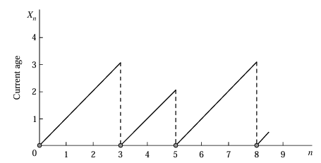
Example 7: Age Process in a Renewal System
A second example of a success run Markov process arises from the current age in a renewal process. Consider a lightbulb whose lifetime, measured in discrete time units, is a random variable \( \tau \) with \[ \Pr(\tau = k) = a_k > 0 \quad \text{for } k = 1, 2, \dots, \quad \sum_{k=1}^{\infty} a_k = 1. \]
Each time a bulb burns out, it is replaced immediately by a new one. Suppose the lifetimes of bulbs are independent and identically distributed as \( \tau \). Let \( X_n \) denote the age of the bulb in service at time \( n \), with \( X_n = 0 \) at failure epochs by convention.
The process \( \{X_n\} \) forms a Markov chain with transition structure similar to that of a success run. The transition probabilities are given by:
\[ p_k = \frac{a_{k+1}}{a_{k+1} + a_{k+2}+ ...}, \quad q_k = 1 - p_k, \quad r_k = 0 \quad \text{for } k \geq 0 \tag{3.45} \]This is interpreted as follows: given the age of the current bulb is \( k \), the conditional probability that it fails in the next time period (i.e., age resets to 0) is \[ \Pr(\text{Failure at } k+1 \mid \text{Survived } k) = \frac{a_{k+1}}{a_{k+1} + a_{k+2}+ ... } = p_k, \] while the probability that it survives to age \( k+1 \) is \( q_k = 1 - p_k \).
Thus, the age process reverts to 0 upon failure and increments by 1 with probability \( q_k \) otherwise, modeling the lifetime evolution of the item under successive renewals.
Last updated: June 15, 2025