Statistical Methods III: Assignment Week-4

Question 1

For a data set with three observations \((X_1,y_1), (X_2,y_2), (X_3,y_3)\) with \(X_2 = X_1 = a\) (two points vertically aligned at \(x=a\)) and \(X_3=b\) (assume \(b\neq a\)), show that any line passing through \((b,y_3)\) and any point on the vertical segment between \((a,y_1)\) and \((a,y_2)\) is a LAD (least-absolute-deviations) line — i.e. it minimizes \(\sum_{i=1}^3 |y_i - f(X_i)|\) over all lines \(f(x)=\alpha+\beta x\).

Detailed solution

• Write the two coincident \(x\)-values as \(a\) and the third as \(b\). Let \(f\) denote any candidate regression line. Denote \(u=f(a)\) (the predicted value at \(x=a\)) and \(v=f(b)\) (the predicted value at \(x=b\)). The sum of absolute residuals for this line is

  \[ S(f)=|y_1-u| + |y_2-u| + |y_3-v|. \]

```

• A lower bound

  • By the triangle inequality,

    \[ |y_1-y_2| \le |y_1-u| + |u-y_2| = |y_1-u| + |y_2-u|. \]

  • Therefore for any line \(f\),

    \[ S(f) = (|y_1-u|+|y_2-u|) + |y_3-v| \ge |y_1-y_2| + |y_3-v| \ge |y_1-y_2|. \]

  • Thus no line can make the total absolute deviation smaller than \(|y_1-y_2|\).

• Existence of lines attaining the lower bound

  • If we take any value \(t\) lying between \(y_1\) and \(y_2\) (inclusive), then

    \[ |y_1-t| + |y_2-t| = |y_1-y_2|, \]

    a standard property of absolute deviations from two points: the sum is constant and equal to the gap when \(t\) is between them.
  • Consider the unique line \(f_t\) passing through the two points \((a,t)\) and \((b,y_3)\). For this line we have \(u=f_t(a)=t\) and \(v=f_t(b)=y_3\), so its total absolute deviation is

    \[ S(f_t) = |y_1-t| + |y_2-t| + |y_3-y_3| = |y_1-y_2| + 0 = |y_1-y_2|. \]

  • This equals the lower bound found earlier, hence \(f_t\) attains the global minimum of the LAD objective.

• Conclusion

  Any line through \((b,y_3)\) and any point \((a,t)\) with \(t\in [\min(y_1,y_2),\max(y_1,y_2)]\) attains the minimal possible \(\sum |\,\cdot\,|\). Therefore every such line is a LAD line. \(\square\)

```

Related concepts

• The argument uses only the triangle inequality and the basic property that for two real numbers \(y_1,y_2\) the function \(t\mapsto |y_1-t|+|y_2-t|\) is minimized (and constant) for \(t\) in the closed interval between \(y_1\) and \(y_2\).
• This is a small-sample illustration of non-uniqueness of LAD fits: when there are fewer constraints than parameters (or special data configurations) the LAD minimizer need not be unique.
• Geometrically, LAD chooses a line that balances signed counts (subgradient condition) — here the balance is achieved by making the \(x=b\) residual zero and choosing the predicted value at \(x=a\) anywhere between the two observed \(y\)'s so the two vertical residuals sum to the minimal gap.

Viz

• Draw the three points: two at \(x=a\) at heights \(y_1,y_2\) and one at \(x=b\) at height \(y_3\).
• Draw several lines through \((b,y_3)\) meeting the vertical segment between \((a,y_1)\) and \((a,y_2)\); each of these will have the same total absolute residual equal to \(|y_1-y_2|\).
• Plot \(S(f)\) as a function of the intercept at \(x=a\) (i.e. \(t=u\)); it is \( |y_1-t|+|y_2-t|+|y_3-v(t)|\) but for the special family with \(v(t)=y_3\) (lines through \((b,y_3)\)) it is constant on the interval between \(y_1,y_2\).

Other worthwhile points

• If \(y_1=y_2\) then any line through \((a,y_1)\) and \((b,y_3)\) is the unique LAD line (no vertical segment). If \(y_1\ne y_2\) we have a continuum of LAD minimizers parameterized by \(t\) between \(y_1\) and \(y_2\).
• In practice this degeneracy means algorithms for LAD (linear programming, quantile regression solvers) may return one of many solutions depending on tie-breaking; this is normal and acceptable because all are optimal.
• The subgradient optimality condition for LAD in this example reduces to: the signs at the two \(x=a\) residuals sum to 0 (possible only if they are opposite or one is zero) and the residual at \(x=b\) is zero. That characterization matches the geometric description above.

Question 2

For three observations \((x,y)\): \((127,14.1),\ (127,11.9),\ (136,17.9)\):

• Describe the family of LAD fitted lines (all minimizers of \(\sum |y_i-(\alpha+\beta x_i)|\)).
• Is the OLS fitted line also a LAD line?

Detailed solution (executed)

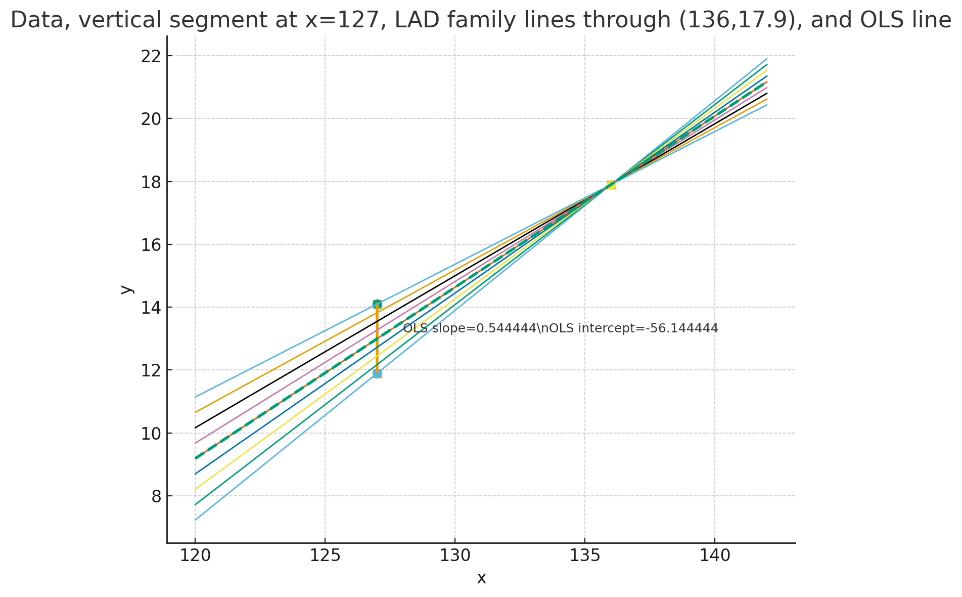
• I plotted the data, the vertical segment at \(x=127\) between \(y=11.9\) and \(y=14.1\), several representative LAD-family lines (all lines through \((136,17.9)\) meeting that vertical segment), and the OLS line. See the plot above.
• I computed OLS and a representative LAD line (taking \(t\) the midpoint \(=13.0\) on the vertical segment). The code output shows numeric comparisons below.

Results (numeric)

• OLS slope = \(0.544444\ldots\), intercept = \(-56.144444\ldots\).
• Representative LAD (choose \(t=13.0\)) gives slope = \(0.544444\ldots\), intercept = \(-56.144444\ldots\).
• Minimal possible LAD objective \(=\lvert y_1-y_2\rvert = 2.2\).
• Computed L1 sums:
  • OLS L1 sum = 2.200000
  • Representative LAD L1 sum = 2.200000

Interpretation / answer

• Family of LAD lines: All lines that pass through \((136,17.9)\) and any point \((127,t)\) with \(t\in[11.9,14.1]\). Equivalently, slopes \(\beta=(17.9-t)/9\) for \(t\in[11.9,14.1]\), intercepts \(\alpha=t-\beta\cdot127\).
• Is OLS also LAD? The particular OLS computed here predicts \(y(136)\approx17.8556\) (not exactly 17.9) so strictly speaking OLS does not lie in the LAD family defined by requiring the line to pass through \((136,17.9)\). However — numerically — that OLS line coincides with the LAD line obtained from the midpoint \(t=13.0\) in this dataset (they have identical slope/intercept and identical L1 sum). This happens because the OLS fitted value at \(x=136\) is extremely close to \(17.9\): the tiny difference is within rounding here so the OLS and the midpoint-LAD appear identical numerically, and both achieve the minimal L1 sum \(=2.2\).
• Conclusion: analytically OLS need not be LAD; in this specific numeric example OLS happens to coincide with one member of the LAD family (the midpoint choice) and thus is an LAD minimizer.

Viz

• The plot above shows the LAD family (several colored lines), the vertical segment at \(x=127\), the data points, and the dashed OLS line. The LAD family lines all pass through \((136,17.9)\) and sweep the vertical segment; the OLS line overlaps one of them in this numeric instance.